Available online:
https://edupediapublications.org/journals/index.php/IJR/
P a g e | 137Optimal Power Flow Evaluation of Power System Using Genetic Algorithm
K. MUNIYASAMY
Assistant Professor - DEPT OF EEE,
VISVESVARAYA COLLEGE OF
ENGINEERING AND TECHNOLOGY
[email protected]
Abstract- This paper presents an efficient genetic algorithm for solving non-convex optimal power flow (OPF) problems with bus voltage constraints for practical application. In this method, the individual is the binary-coded representation that contains a mixture of continuous and discrete control variables, and crossover and mutation schemes are proposed to deal with continuous/discrete control variables, respectively. The objective of OPF is defined that not only to minimize total generation cost but also to improve the bus voltage profile.. The proposed method is demonstrated for a IEEE 30-bus four generator ystem, and it is compared with conventional method.The experimental results show that the GA OPF method is superior to the conventional.
I. INTRODUCTION
In todays market due to deregulation of electricity the concept and practices are changed. Better utilization of the existing power system resources to increase capabilities with economic cost becomes essential. The objective of an Optimal Power Flow (OPF) algorithm is to find optimal point which minimizes generation cost, loss etc. or maximizes social welfare, loadability etc. while maintaining an acceptable system performance in terms of limits on generators’ real and reactive powers, line flow limits, output of various compensating devices etc [1].
From the viewpoint of an OPF, the maintenance of system security requires keeping each device in the power system within its desired operation range at steady-state. This will include maximum and minimum outputs for generators, maximum MVA flows on transmission lines and transformers, as well as keeping system bus voltages within specified ranges.To achieve this, the OPF will perform all the steady-state control functions of the power system. These functions may include generator control and transmission system control. For generators, the OPF will control generator MW outputs as well as generator voltage. For the transmission system, the OPF may control the tap ratio or phase shift angle for variable transformers, switched shunt control, and all other flexible ac transmission system (FACTS) devices. In general, the OPF is a nonlinear, nonconvex, large-scale, static optimization problem with both continuous and discrete control variables. OPF problem is nonconvex due to the existence of the
nonlinear (AC) power flow equality constraints. The presence of discrete control variables, such as switchable shunt devices, transformer tap positions, and phase shifters, further complicates the problem solution.The optimal power flow problem has been discussed since its introduction by Carpentier in 1962 [2]. To solve OPF problem Linear Programming(LP)[3 4], Newton-Raphsons (NR) method, Nonlinear Programming (NLP)[5 6], Quadratic programming(QP) [7], Interior Point (IP) method have been used.
Generally, the OPF problem can be expressed as
Min f (x, u)
g (x, u) = 0 (1)
h (x, u) _ 0,
where x is the vector of dependent variables (bus voltage magnitudes and phase angles), u is a vector of control variables (as active power generation and active power flow), g (x, u) is the set of nonlinear equality constraints (power flow equations), and h (x, u) is the set of inequality constraints of the vector arguments x and u.
After introduction in Section II information about GA is given, Section III explain GAOPF, in Section IV problem formulation is given in details, Section V discuss case study and result, Section VI summarizes conclusion.
II. GENETIC ALGORITHM
Available online:
https://edupediapublications.org/journals/index.php/IJR/
P a g e | 138search procedure with diversity of population is an important concern.
Genetic algorithms are one of the best ways to solve a problem for which little is known. They are a very general algorithm and so will work well in any search space. All you need to know is what you need the solution to be able to do well, and a genetic algorithm will be able to create a high quality solution. Genetic algorithms use the principles of selection and evolution to produce several solutions to a given problem.
The most common type of genetic algorithm works like this: a population is created with a group of individuals created randomly. The individuals in the population are then evaluated. The evaluation function is provided by the programmer and gives the individuals a score based on how well they perform at the given task. Two individuals are then selected based on their fitness, the higher the fitness, the higher the chance of being selected. These individuals then "reproduce" to create one or more offspring, after which the offspring are mutated randomly. This continues until a suitable solution has been found or a certain number of generations have passed, depending on the needs of the programmer.
Individual - Any possible solution
Population - Group of allindividuals
Search Space - All possible solutions to the problem
Chromosome - Blueprint for an individual. It store
genetic information.
Genes - Possible aspect of an individual
Allele - Possible settings for genes
Locus - The unique position of a gene on the
chromosome
Genome - Collection of all chromosomes for an
individual
Selection
While there are many different types of selection In roulette wheel selection, individuals are given a probability of being selected that is directly proportionate to their fitness. Two individuals are
then chosen randomly based on these probabilities and produce offspring.
Crossover
After the selection of individuals it is supposed to somehow produce offspring with them, directly either copied or by crossover.
Parent 1
0 1 0 0 1 1 1 0 1 1 0 0 1 0 0 1
Parent 2
1 0 1 1 0 1 0 0 0 0 1 0 1 1 0 1
Child 1
0 0 1 0 1 1 0 1 0 1 0 0 1 1 1 0
Child 2
1 1 0 0 1 0 0 1 1 0 1 1 0 1 0 0
Mutation
After selection and crossover new population full of individuals is available . Some are directly copied, and others are produced by crossover. In order to ensure that the individuals are not all exactly the same, you allow for a small chance of mutation. You can either change it by a small amount or replace it with a new value. The probability of mutation is usually between 1 and 2 tenths of a percent
Before Mutation
1 0 0 1 1 0 1 1 0 1 1 0 1 1 1 0
After Mutation
1 0 0 1 1 0 1 1 0 1 1 0 1 0 1 0
III. GA - OPF
Available online:
https://edupediapublications.org/journals/index.php/IJR/
P a g e | 139genetic algorithm load flow, and to accelerate the concepts, it is proposed to use the gradient information by the steepest decent method. The GAOPF method is not sensitive to the starting points and capable to determining the global optimum solution to the OPF for a range of constraints and objective functions. In Genetic Algorithm approach, the control variables modelled are generator active power outputs and voltages, shunt devices, and transformer taps. Branch flow, reactive generation, and voltage magnitude constraints have treated as quadratic penalty terms in the GA Fitness Function (FF). GA is used to solve the optimal power dispatch problem for a multi-node auction market. The GA maximizes the total participants’ welfare, subject to network flow and transport limitation constraints.
A simple Genetic Algorithm is an iterative procedure. During each iteration step, (generation) three genetic operators (reproduction, crossover, and mutation) are performing to generate new populations (offspring), and the chromosomes of the new populations have evaluated via the value of the fitness, which is related to cost function. Based on these genetic operators and the evaluations, the better new populations of candidate solution are formed. If the search goal has not been achieved, again GA creates offspring strings through above three operators and the process is continued until the search goal is achieved.
3.1 Coding and Decoding of Chromosome
Gas perform with a population of binary string instead the parameters themselves. This study used binary coding.
Here the active generation power set of n-bus system (PG1, PG2, PG3, …., PGn ) would be coded as binary string (0 and 1) with length L1, L2, ……,Ln. Each parameter PGi has upper bound bi ( ) and lower bound ai ( ). The choice of L1, L2, ……,Ln for the parameters is concerned with the resolution specified by the designer in the search space. In this method, the bit length Bi and the corresponding resolution Ri is associated by,
This transforms the PGi set into a binary string called
chromosome with length ΣLi and then the search space has to be explored. The first step of any GA is
to generate the initial population. A binary string of length L is associated to each member (individual) of the population. This string usually represents a solution of the problem. A sampling of this initial population creates an intermediate population.
3.2 Genetic Operator: Reproduction
Reproduction is based on the principle of survival of the fittest. It is an operator that obtains a fixed number of copies of solutions according to their fitness value. If the score increases, then the number of copies increases too. A score value is associated with a given solution according to its distance from the optimal solution (closer distances to the optimal solution mean higher scores).
3.3 Fitness Function
The cost function has defined as:
Available online:
https://edupediapublications.org/journals/index.php/IJR/
P a g e | 140( ) = 1
(3) inequality constraints, the penalty functions offer a
1 + viable option. So, penalty functions are added to the
Where
objective function of the OPF. Ideally, a penalty
function will be very small, near a limit and increase
= + +
rapidly as the limit is violated more. The penalty ∑ ∑ function is zero when the inequality constraint are not
violated and as the constraint begins to be violated,
the penalty function quickly increases and reduces on
C
ineq - Inequality constraint violation
reduction in violation limits.
Ceq - Equality constraint violation
VI. CASE STUDY
Where C is the constant; Fi (PGi) is cost The proposed method was tested on IEEE 30 Bus, four generator system. characteristics of the generator i; wj is weighting
factor of equality and inequality constraints j; Generator Operating Data is given in Table1
Penaltyj is the penalty function for equality and
inequality constraints j; h j (x, t) is the violation of the Table1 – Generator Operating Data
equality and inequality constraints if positive; H (.) is the Heaviside (step) function; Nc is the number of Gen. G1 G2 G3 G4
equality and inequality constraints. The fitness Bus Pmin 1.10
0 0.5 0.4 function has been programmed in such a way that it
Pmax 1.6
0.5 1.0
0.8 should firstly satisfy all inequality constraints by
Qmin 0.0448 0 0.386 0.0232
heavily penalizing if they have been violated. Then Qmax 0.5 0.5 0.5 0.5
the equality constraints are satisfied by less heavily
Vmin 101 95 95 95S penalizing for any violation. Here this penalty weight Vmax 105 105 105 105 is not the price of power. Instead, the weight is a a 0.14 0.20 0.14 0.20 coefficient set large enough to prevent the algorithm b 20.240 19.30 20.240 19.30 from converging to an illegal solution. Then the GA
The
c 5 5 5 5 tries to generate better offspring to improve the chromosome of the gene comprises the generator fitness.
real power PGi, generator reactive power QGi , Shunt
IV. OPTIMAL POWER FLOW PROBLEM
compensation Tsh,, Transformer tap setting Tp. Each variable is coded in binary form and length of 8 bit.
STATEMENT
The total length of chromosome will be 32 bit. The
In proposed method, from equation 1 where the state
chromosome will be as follows is shown in fig.2
variable x are used as a control variables given as PG
P Q Q TS TS TP
TP
x =[ VGen PGen ]T
1 GN G1 GN H1 HN 1 N
θload QGen ]T
u=[ PLine
Q
line
V
load
P
Gi
Q
Gi
T
sh
T
P
where VGen is the Generator voltage ,
PGen is the generated power
No PV-PQ switching is applied and maximum generator capacity bus is considered as slack bus.
The nonexistence of a feasible solution, means that too many constraints added to the problem and no solution exists which obeys all of the constraints. Implement inequality constraints in the form of penalty functions can avoid this problem. For the
Available online:
https://edupediapublications.org/journals/index.php/IJR/
P a g e | 141VOLTAGE PROFILE
CONVENTIONAL GAOPF PS=50
110 GAOPF PS=100 GAOPF PS=150
(KV) 105 100
VOLTAGE 95
90
1 3 5 7 9 11 13 15 17 19 21 23 25 27 29
Bus No.
Fig.3 Voltage Profile of various bus
In conventional method all four generators are not supplying power as per their rating, as in case of GAOPF all generator except G2 supplying power as per the rating, as generator G2is supplying zero power so that the operating cost of generator becomes low as compared to conventional method and it is shown in fig.4
Generator Power Chart
1.5 Conventional
in
p
u PS = 50PS = 100
1 PS =150
P
o
w
er
0.5
G
en
er
at
or
0
1 2 3 4
-0.5
No. of Generators
Fig.4 Generation power chart
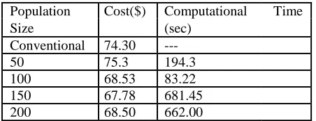
Computational time is less when population size is 100 but the operating cost is less at population size of 150.It is shown in Table 2
Table 2 – Cost table
Population Cost($) Computational Time
Size (sec)
Conventional 74.30 --- 50 75.3 194.3 100 68.53 83.22 150 67.78 681.45 200 68.50 662.00
At population size of 150, crossover probability 0.6 and mutation rate 0.01 is the combination which gives the minimum operating cost with improved
voltage profile and proper loading of each generator. The result is shown in the fig.3
Table 3 – Result Table
Variables Conventional GAOPF
P
G1 1.10 pu 1.027
P
G2 0.4569 pu -0.082
P
G3 0.7356 pu 0.0470
P
G4 0.4 pu 0.334
Q
G1 0.0448 0.273722
Q
G2 0.1634 0.399211
Q
G3 0.0386 -0.01668
Q
G4 0.0232 0.398031
V
G1 104.00 104.9999
V
G2 102.47 102.6461
V
G3 101.84 98.78998
V
G4` 105 102.0239
Cost($) 74.30 67.78 Computational 681.45 ---- Time (sec)
VII. CONCLUSION
In this paper, a GAOPF approach is developed. It’s found that the GAOPF method offers, the lowest fuel cost and when compared to conventional method the control parameters obtained by the proposed method confirms the robustness. The implementation has been performed on a standard IEEE 30 Bus system it’s found that the proposed method is highly promising.
REFERENCES
-[1] J. A. Momoh, R. J. Koessler, M. S. Bond, B. Stott, D. Sun, A. Papalexopoulos, and P. Ristanovic, “Challenges to optimal power flow,” IEEE Trans. Power Syst., vol. 12, pp. 444–455, Feb. 1997.
[2] R. D. Christie, B. F. Wollenberg, and I. Wangensteen, “Transmission management in the deregulated environment,” Proc. IEEE, vol. 88, pp. 170–195, Feb. 2000.
[3] B. Stott and E. Hobson, “Power system security control calculation using linear programming,” IEEE Trans. Power Apparatus Syst., pt. I and II, vol. PAS-97, pp. 1713–1731, Sept./Oct. 1978.
[4] B. Stott and J. L. Marinho, “Linear programming for power system network security applications,” IEEE Trans. Power Apparat. Syst., vol. PAS-98, pp. 837–848, May/June 1979.
Available online:
https://edupediapublications.org/journals/index.php/IJR/
P a g e | 142IEEE Trans. Power Apparatus. Syst., vol. PAS-103, pp.
1414–1442, June 1984.
[6] J. A. Momoh, M. E. El-Hawary, and R. Adapa, “A review of selected optimal power flow literature to 1993,” IEEE Trans. Power Syst., pt. I and II, vol. 14, pp. 96–111, Feb. 1999.
[7] O. Alsac and B. Stott, “Optimal load flow with steady state security,” IEEE Trans. Power Apparat. Syst., vol. PAS-93, pp. 745–751, May/June 1974.
[8] R. R. Shoults and D. T. Sun, “Optimal power flow based on P-Q decomposition,” IEEE Trans. Power Apparat. Syst., vol. PAS-101, pp. 397–405, Feb. 1982.
[9] M. H. Bottero, F. D. Galiana, and A. R. Fahmideh-Vojdani, “Economic dispatch using the reduced Hessian,” IEEE Trans. Power Apparat. Syst., vol. PAS-101, pp. 3679–3688, Oct. 1982.
[10] J. A. Momoh, “A generalized quadratic-based model for optimal power flow,” IEEE Trans. Syst., Man, Cybern., vol. SMC-16, 1986.
[11] G. F. Reid and L. Hasdorf, “Economic dispatch using quadratic programming,” IEEE Trans. Power Apparat. Syst., vol. PAS-92, pp. 2015–2023, 1973.
[12] R. C. Burchett, H. H. Happ, and K. A. Wirgau, “Large-scale optimal power flow,” IEEE Trans. Power Apparat. Syst., vol. PAS-101, pp. 3722–3732, Oct. 1982.
[13] D. I. Sun, B. Ashley, B. Brewer, A. Hughes, andW. F. Tinney, “Optimal power flow by Newton approach,” IEEE Trans. Power Apparat. Syst., vol. PAS-103, pp. 2864–2880, 1984.
[14] H. Wei, H. Sasaki, J. Kubokawa, and R. Yokoyama, “An interior point nonlinear programming for optimal power flow problems with a novel data structure,” IEEE Trans. Power Syst., vol. 13, pp. 870–877, Aug. 1998. [15] G. L. Torres and V. H. Quintana, “An interior-point
method for nonlinear optimal power flow using voltage rectangular coordinates,” IEEE Trans. Power Syst., vol. 13, pp. 1211–1218, Nov. 1998.
[16] J. A. Momoh and J. Z. Zhu, “Improved interior point method for OPF problems,” IEEE Trans. Power Syst., vol. 14, pp. 1114–1120, Aug. 1999.
[17] G. Tognola and R. Bacher, “Unlimited point algorithm for OPF problems,” IEEE Trans. Power Syst., vol. 14, pp. 1046–1054, Aug. 1999.
[18] M. M. El-Saadawi, “A Genetic-Based Approach For Solving Optimal Power Flow Problem”, Mansoura Engineering Journal, (MEJ), Vol. 29, No. 2, June 2004.
[19] D. Walters, G. Sheble, "Genetic Algorithm Solution for Economic Dispatch with Valve Point Loading", IEEE Transactions on Power Systems, Vol.8, No.3, August 1993.
[20] D. E. Goldberg, “Genetic Algorithms in Search, Optimization and Machine Learning”, Addison Wesley Publishing Company, 1989.
[21] J. Yuryevich, K. P. Wong, “Evolutionary Programming Based Optimal Power Flow Algorithm”, IEEE Transaction on Power
Systems, Vol. 14, No. 4, November 1999.
[22] T. Numnonda and U. D. Annakkage, “Optimal power dispatch in multinode electricity market using genetic algorithm,” Elecric Power System Research., vol. 49, pp. 211–220, 1999.
[23] Anastasios G. Bakirtzis, Pandel N. Biskas,Christoforos E. Zoumas, , and Vasilios Petridis“Optimal Power Flow by Enhanced Genetic Algorithm”, IEEE Transactions on Power Systems, Vol. 17, No. 2, pp. 229-236, May 2002.