Three Essays on Structural Models

(1)

Scholarship@Western

Electronic Thesis and Dissertation Repository

5-29-2018 11:00 AM

Three Essays on Structural Models

Xinghua Zhou

The University of Western Ontario

Supervisor Reesor, Mark

The University of Western Ontario

Graduate Program in Applied Mathematics

A thesis submitted in partial fulfillment of the requirements for the degree in Doctor of Philosophy

Follow this and additional works at: https://ir.lib.uwo.ca/etd

Part of the Corporate Finance Commons, Finance and Financial Management Commons, and the

Other Applied Mathematics Commons

Recommended Citation Recommended Citation

Zhou, Xinghua, "Three Essays on Structural Models" (2018). Electronic Thesis and Dissertation Repository. 5427.

https://ir.lib.uwo.ca/etd/5427

This Dissertation/Thesis is brought to you for free and open access by Scholarship@Western. It has been accepted for inclusion in Electronic Thesis and Dissertation Repository by an authorized administrator of

(2)

Abstract

My thesis includes three papers on contingent claims valuation of corporate securities using structural models of credit risk. Our study focuses on structural models and their applications in estimating damages in security class actions, option pricing and warrant pricing.

Securities class actions typically involve some misrepresentation by a firm that overstates its true value. In securities class actions econometric models are used to assess damages to shareholders. However, studies on measuring damages for debt-holders are limited. My first paper uses a modified Merton framework to measure the impact of misrepresentation on the value of other components (e.g., debt, warrants) of a firm’s capital structure. Using structural models and leveraging the relationship between equity and firm value, we use observable eq-uity information to determine firm value and hence the effect of misrepresentation on value of other securities in the capital structure. We investigate various capital structures and show that misrepresentation can have a significant impact on the value of all components in the capital structure. We find that the misrepresentation impact on debt value depends on firm leverage and debt seniority and not on the warrant dilution factor. Generally, the debt for higher-leverage firms is more sensitive to the misrepresentation impact than for lower-leverage firms and junior debt is more affected by fraud than senior debt. The impact on warrant value is determined by warrant moneyness (stock price), with the dilution factor having no effect.

My second paper extends the study in my first paper into the First Passage Time (FPT) framework, which is capable of modeling firms with complex debt structures. Our findings have important consequences for damages assessment and allocation of settlement awards in securities class actions. In some jurisdictions damages awarded are net of any hedge or risk-limitation transaction. Since corporate securities such as bonds and stocks are often held in portfolios for hedging purposes, measuring the effect of misrepresentation on all of the firm’s issuances is essential to accurately computed damages awards. In addition to our main findings, we explicitly discuss bankruptcy costs for the First Passage Time model. Furthermore, we are able to reduce a system of two non-linear equations, used to connect the unobservable firm value and firm value volatility to observable equity value and equity volatility, into one equation. This technique improves the ability to solve the non-linear system.

My third paper studies option and warrant pricing under the structural framework (both Merton and FPT frameworks). We study the calibration of structural frameworks using a mar-ket implied volatility skew. We show that the model implied volatility skew under FPT frame-work is much more flexible than that under the Merton frameframe-work. Moreover, we extend the FPT structural framework to include warrants into the firm’s capital structure. Using historical market data, we show the pricing model (for both options and warrants) under FPT framework significantly outperforms the pricing models under Merton framework.

Keywords:Damages; Misrepresentation; Securities Class Actions; Capital Structure; Debt; Warrants; Merton Model; Connection Between Unobservable Firm Value and Observable Stock Price; Structural Models; Pricing; Valuation With Observable Information; Volatility Skew; Warrants Pricing;

(3)

All three of my papers included in this thesis are co-authored with my Supervisor R. Mark Reesor. I, Xinghua Zhou, am the primary author.

(4)

Acknowlegements

I would like to thank first and foremost my supervisor Prof. Mark Reesor for his intellectual mentorship, invaluable guidance and great support during my Ph.D. study. I would like to thank Prof. Matt Davison, Prof. Adam Metzler, Prof. Rogemar Mamon, Prof. Walid Busaba, Prof. Pascal Francois, and Prof. Fredrik Odegaard for their helpful suggestions and discus-sions. I would like to thank Audrey Kager, Cory Walton, and all the faculty and stafffrom the Department of Applied Mathematics who have supported me over the years. Last but not least, I would like to thank my parents, my family and friends who have provided love, patience, and encouragement throughout this long process.

(5)

List of Figures

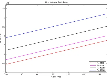
2.1 Firm value versus stock price for the debt and equity capital structure. F is the face value of the debt and the parameter inputs areσS ₌ ₀_._3,

T − t = 5,

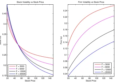
r=0.03, andN =100. . . 26 2.2 Left panel is stock price volatility versus stock price (for fixed firm value

volatility) and right panel is firm value volatility versus stock price (for fixed

σS = ₀._{3) for the debt and equity capital structure.} _F _{is the face value of the}

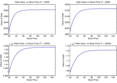
debt and the parameter inputs areT −t= 5,r= 0.03, andN =100. . . 27 2.3 Debt value versus stock price for the debt and equity capital structure (fixed

stock price volatility). The panels correspond to different debt face values and the parameter inputs areσS =₀._3,

T −t= 5,r=0.03, andN =100. . . 28 2.4 Debt value versus stock price for the debt and equity capital structure (fixed

firm value volatility). The panels correspond to different debt face values and the parameter inputs areT−t= 5,r= 0.03, andN =100. Firm-value volatility is computed usingSt =50 andσS =0.3. . . 29

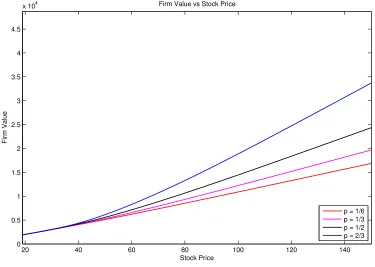
2.5 Firm value versus stock price for the warrants and common shares capital struc-ture. pis the dilution factor and the parameter inputs areσS =₀._3,_T

W−t= 2,

r=0.03,K = 60 andN =100. . . 30 2.6 Warrant value versus stock price for the warrants and common shares capital

structure (constant firm value volatility). pis the dilution factor and the param-eter inputs areTW−t= 2,r =0.03,K =60 andN = 100. Firm-value volatility

is computed usingSt =50 andσS =0.3. . . 31

2.7 Left panel is stock price volatility versus stock price (fixed firm value volatil-ity) and right panel is firm-value volatility versus stock price (fixed stock price volatility) for the warrants and common shares capital structure. p is the di-lution factor and the parameter inputs areT −t = 5, r = 0.03, and N = 100. Firm-value volatility for the right panel is computed usingSt =50 andσS =0.3. 32

2.8 Left and right panels are firm value versus stock price (fixed firm value volatil-ity) for the debt, warrant and common shares capital structure for p= 1/6 and

p = 1/2, respectively. F is the face value of the debt and the parameter inputs areT −t = 5,r = 0.03, andN = 100. Firm-value volatility is computed using

St =50 andσS =0.3. . . 33

2.9 Debt value versus stock price for the debt, warrant and common shares capital structure (fixed firm-value volatility). The panels correspond to different debt face values and the parameter inputs areT − t = 5, r = 0.03, and N = 100. Firm-value volatility is computed usingSt = 50 andσS = 0.3. . . 34

(9)

volatility) for the debt, warrant and common shares capital structure for p =

1/6 andp=1/2, respectively. Fis the face value of the debt and the parameter inputs areT −t= 5,r= 0.03, andN =100. Firm-value volatility is computed usingSt =50 andσS =0.3. . . 35

2.11 Left and right panels are stock price volatility versus stock price (for fixed firm value volatility) for the debt, equity, and common shares capital structure for

p = 1/6 and p = 1/2, respectively. F is the face value of the debt and the parameter inputs areT −t= 5,r =0.03, andN = 100. Firm-value volatility is computed usingSt = 50 andσS = 0.3. . . 36

2.12 Left and right panels plot D_D˜ versusδfor the debt and equity capital structure for

St = 50 andSt = 125, respectively. Lines in each plot correspond to different

debt face values, F, and the parameter inputs are T −t = 5, r = 0.03, and

N = 100. . . 37 2.13 True/fraudulent value ratios of junior (left panels) and senior (right panels)

debt as a function ofδ forSt = 50 (top panels) andSt = 125 (bottom panels),

respectively, for the junior and senior debt and equity capital structure. Lines in each plot correspond to different debt face values,F, and the parameter inputs areT −t=5,r =0.03, andN = 100. . . 38 2.14 Left and right panels plot W_W˜ versusδfor the warrant and common shares capital

structure forSt = 50 andSt = 125, respectively. Lines in each plot correspond

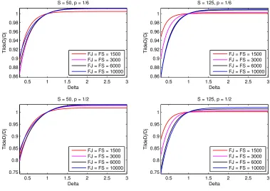
to different dilution factors,p, and the parameter inputs areT−t =5,r=0.03, andN =100. . . 39 2.15 D_D˜ versus δ for St = 50 (left panels), St = 125 (right panels), p = 1/6 (top

panels) and p = 1/2 (bottom panels), respectively, for the debt, warrants and common shares capital structure. Lines in each plot correspond to different debt face values, F, and the parameter inputs are T −t = 5, r = 0.03, and

N = 100. . . 40

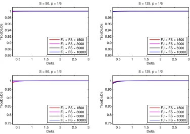
2.16 W_W˜ versus δ for St = 50 (left panels), St = 125 (right panels), p = 1/6 (top

panels) and p = 1/2 (bottom panels), respectively, for the debt, warrants and common shares capital structure. Lines in each plot correspond to different debt face values, F, and the parameter inputs are T −t = 5, r = 0.03, and

N = 100. . . 41 2.17 True/fraudulent value junior debt ratios as a function ofδforSt =50 (left

pan-els),St =125 (right panels), p=1/6 (top panels) andp=1/2 (bottom panels),

respectively, for the junior and senior debt, warrants and common shares capi-tal structure. Lines in each plot correspond to different debt face values,F, and the parameter inputs areT −t =5,r= 0.03, andN =100. . . 42 2.18 True/fraudulent value senior debt ratios as a function ofδforSt =50 (left

pan-els),St =125 (right panels), p=1/6 (top panels) andp=1/2 (bottom panels),

respectively, for the junior and senior debt, warrants and common shares capi-tal structure. Lines in each plot correspond to different debt face values,F, and the parameter inputs areT −t =5,r= 0.03, andN =100. . . 43

(10)

2.19 Value line of commom shares - The period between the two vertical lines in is the class period. The blue solid line shows the historical stock price of AEM from January 2010 to December 2011. The stock price value line, represented by the red dashed line, is constructed by the event study approach discussed in Section 2.1.1 . . . 44

2.20 Value line of warrants - The period between the two vertical lines in is the class period. The blue solid line shows the historical warrant price of AEM from January 2010 to December 2011. The warrant price value line, represented by the magenta dashed line, is calculated by the methodology discussed in Section 2.5 . . . 45

2.21 Damages Ribbon of Debt - The red line and blue line show the damages ribbons of debt computed using the Merton model and the FPT model, respectively, during the period from April 7, 2010 to October 18, 2011. . . 46

3.1 Firm Value and Capital Structure - Firm value VtF versus equity value EQt,

debt valueDt and the sum ofEQt andDt using the model in Section 3.2. The

bankruptcy costsBCt are the difference betweenVtF andDt +EQt. Parameters

are:σF = _21%,_r =_5%,_T₋_t=_5,_K = _{50, and}_w= ₄₈._{67% (parameter values}

randware choosen following Huang and Huang[29]). . . 56

3.2 Effect of Fraud on Debt Value (FPT) - Fraud size,δ, versus junior/senior zero coupon debt in the left/right panel using the First Passage Time model in Sec-tion 3.2. The junior and senior debts have the same maturity date. The quasi-leverageLis defined as quasi market value of debt to the quasi asset value, i.e.,

L = (e−r(T−t)K)/(EQt +e−r(T−t)K). The initial equity value is 100, we use the

quasi-leverage ratio to compute the corresponding debt face valueK. The face value for junior debt and senior debt are the same, i.e., Kj = Ks = K/2. Fol-lowing the empirical results in Schaefer and Strebulaev[47], we set the leverage ratioLand equity volatilityσE _{as 0}._{10, 0}._{32, and 0}._{50 and 25%, 31%, and 42%}

for AAA, A, and BB credit rating firms, respectively. The rest of the parameter values arer = 5%, T − t = 5, wj = 82.9%, and ws = 50.9% (the loss given defaultwfollows [42]). . . 65

3.3 Effect of Fraud on Debt Value (SD) - Fraud size, δ, versus junior/senior zero coupon debt in the left/right panel using the Subordinated Debt model. The junior and senior debts have the same maturity date. The quasi-leverage L

is defined as quasi market value of debt to the quasi asset value, i.e., L =

(e−r(T−t)F)/(EQt+e−r(T−t)F). The initial equity value is 100, we use the

quasi-leverage ratio to compute the corresponding debt face valueF. The face value for junior debt Fj _{and senior debt} _Fs _{are the same, i.e.,}_Fj = _Fs = _F/_2.

Fol-lowing the empirical results in Schaefer and Strebulaev[47], we set the leverage ratioLand equity volatilityσE as 0.10, 0.32, and 0.50 and 25%, 31%, and 42% for AAA, A, and BB credit rating firms, respectively. The rest of the parameter values arer= 5%, andT −t =5. . . 66

(11)

class period. The blue line shows the historical stock price of AEM from Jan-uary 2010 to December 2011. The value line of stock, which is represented by the red dash line, is constructed by the event study approach (see Section 3.1.1). 67 3.5 Notes Damages Ribbon - The graph shows the damages ribbon of notes during

the period from April 7, 2010 to October 18, 2011. . . 68

4.1 First-passage-time model implied volatility skew - Moneyness of stock priceκ versus implied stock volatilityν. Parameters input are below: r = 5%, t = 0,

TO = 0.33, ¯T = 5, L = 38.5%, and σF = 30% ( The range of parameter

inputs L and κ are choosen following Geske, Subrahmanyam and Zhou[15]. The leverage L∗_{in their paper is approximately equal to} _L∗_er( ¯T−t) _{in ours, i.e.,}

L= L∗er( ¯T−t)_{). . . 79}

4.2 Merton model implied volatility skew - Moneyness of stock priceκversus im-plied stock volatilityν. Parameters input are below: r= 5%,t =0,TO =0.33,

¯

T = 5, L = 38.5%, and σF = _{30% ( The range of parameter inputs} _L _andκ

are choosen following Geske, Subrahmanyam and Zhou[15]. The leverageL∗

in their paper is approximately equal toL∗_er( ¯T−t)_{in ours, i.e.,}_L= _L∗_er( ¯T−t)_{). . . . 80}

4.3 First-passage-time model - Moneyness of stock price κ versus Moneyness of firm valueα. Parameters input are below: r = 5%,t = 0, TO = 0.33, ¯T = 5,

L= 38.5%, andσF = _{30% ( The range of parameter inputs}_L_andκ_{are choosen}

following Geske, Subrahmanyam and Zhou[15]. The leverageL∗in their paper is approximately equal toL∗er( ¯T−t)in ours, i.e.,L= L∗er( ¯T−t)). . . 81 4.4 Merton model - Moneyness of stock price κ versus Moneyness of firm value

α. Parameters input are below: r = 5%, t = 0, TO = 0.33, ¯T = 5, L =

38.5%, and σF = _{30% ( The range of parameter inputs}

L and κ are choosen following Geske, Subrahmanyam and Zhou[15]. The leverageL∗_{in their paper}

is approximately equal toL∗er( ¯T−t)in ours, i.e.,L= L∗er( ¯T−t)). . . 82 4.5 Frim Value and Capital Structures - Firm value VF

t versus warrant value Xt,

equity valueEQt, debt valueDtand the sum ofXt,EQtandDt. The bankruptcy

costsBCtare the difference betweenVtF andDt+EQt+Xt. Parameters input are

below: σF = _21%, _r = _5%,_t = _0,_T

W = 1, T = 5, K = 50, KW = 5, N = 10,

M = 3 and w = 48.67% ( parameter inputs r and w are choosen following Huang and Huang[17]). . . 84 4.6 First-passage-time warrant model implied volatility skew - Moneyness of stock

priceκversus implied stock volatilityv. Parameters input are below: p=20%

r = 5%, t = 0, TW = 1, ¯T = 5, L = 38.5%, and σF = 30% ( The range

of parameter inputsLandκare choosen following Geske, Subrahmanyam and Zhou[15]. The leverageL∗in their paper is approximately equal toL∗er( ¯T−t)_in

ours, i.e.,L= L∗er( ¯T−t)). . . 89 4.7 First-passage-time warrant model - Moneyness of stock priceκversus

Money-ness of firm valueα. Parameters input are below: p = 20% r = 5%, t = 0,

TW = 1, ¯T = 5, L = 38.5%, and σF = 30% ( The range of parameter inputsL

andκare choosen following Geske, Subrahmanyam and Zhou[15]. The lever-ageL∗in their paper is approximately equal toL∗er( ¯T−t)_{in ours, i.e.,}_L₌ _L∗

er( ¯T−t)_{). 90}

(12)

4.8 Merton warrant model implied volatility skew - Moneyness of stock price κ versus implied stock volatilityv. Parameters input are below: p= 20%r= 5%,

t = 0, TW = 1, ¯T = 5, L = 38.5%, andσF = 30% ( The range of parameter

inputs L and κ are choosen following Geske, Subrahmanyam and Zhou[15]. The leverage L∗in their paper is approximately equal to L∗er( ¯T−t) in ours, i.e.,

L= L∗_er( ¯T−t)_{). . . 91}

4.9 Merton warrant model - Moneyness of stock priceκversus Moneyness of firm valueα. Parameters input are below: p= 20%r = 5%,t = 0,TW = 1, ¯T = 5,

L= 38.5%, andσF = _{30% ( The range of parameter inputs}_L_andκ_{are choosen}

following Geske, Subrahmanyam and Zhou[15]. The leverageL∗in their paper is approximately equal toL∗_er( ¯T−t)_{in ours, i.e.,}_L= _L∗_er( ¯T−t)_{). . . 92}

4.10 Call option under first-passage time model with warrant implied volatility skew - Moneyness of stock price κ versus implied stock volatility v. Parameters input are below: p = 20% r = 5%, t = 0, TO = 0.33, TW = 1, ¯T = 5,

L= 38.5%, andσF = 30% ( The range of parameter inputsLandκare choosen following Geske, Subrahmanyam and Zhou[15]. The leverageL∗_{in their paper}

is approximately equal toL∗er( ¯T−t)_{in ours, i.e.,}_L₌ _L∗

er( ¯T−t)_{). . . 95}

4.11 Call option under first-passage time model with warrant - Moneyness of stock priceκ versus Moneyness of firm value α. Parameters input are below: p =

20% r = 5%, t = 0,TO = 0.33, TW = 1, ¯T = 5, L = 38.5%, and σF =

30% ( The range of parameter inputs L and κ are choosen following Geske, Subrahmanyam and Zhou[15]. The leverageL∗in their paper is approximately equal toL∗er( ¯T−t) in ours, i.e.,L= L∗er( ¯T−t)). . . 96 4.12 Call option under Merton model with warrant implied volatility skew -

Mon-eyness of stock priceκversus implied stock volatilityv. Parameters input are below: p = 20% r = 5%, t = 0, TO = 0.33, TW = 1, ¯T = 5, L = 38.5%,

andσF = _{30% ( The range of parameter inputs} _L_and κ _{are choosen}

follow-ing Geske, Subrahmanyam and Zhou[15]. The leverage L∗ in their paper is approximately equal toL∗er( ¯T−t) in ours, i.e.,L= L∗er( ¯T−t)). . . 97 4.13 Call option under Merton model with warrant - Moneyness of stock price κ

versus Moneyness of firm valueα. Parameters input are below: p = 20%r =

5%,t = 0,TO = 0.33,TW = 1, ¯T = 5, L = 38.5%, and σF = 30% ( The range

of parameter inputsLandκare choosen following Geske, Subrahmanyam and Zhou[15]. The leverageL∗in their paper is approximately equal toL∗er( ¯T−t)in ours, i.e.,L= L∗_er( ¯T−t)_{). . . 98}

4.14 Fitting Market Implied Volatility Skew using Three Options - The cross mark-ers are the Black-Scholes implied volatilities from the option prices observed from the market. Especially, the red cross markers are the three market im-plied stock volatility used to calibration the structural model for both the First Passage Time framework and the Merton framework. The blue line is the cal-ibrated volatility skew using the option pricing model under the First Passage Time framework while the green line is output from the option pricing model under the Merton framework. The market data is the mid-price of call options on Apple’s share on date 2009-03-25. The options’ time to maturity is 206 days. 106

(13)

ers are the Black-Scholes implied volatilities from the option prices observed from the market. Especially, the red cross markers are the three market im-plied stock volatility used to calibration the structural model for both the First Passage Time framework and the Merton framework. The blue line is the cal-ibrated volatility skew using the option pricing model under the First Passage Time framework while the green line is output from the option pricing model under the Merton framework. The market data is the mid-price of call options on Apple’s share on date 2009-10-02. The options’ time to maturity is 50 days. 107

4.16 Fitting Market Implied Volatility Skew using Two Options - The cross markers are the Black-Scholes implied volatilities from the option prices observed from the market. Especially, the red cross markers are the two market implied stock volatility used to calibration the structural model for both the First Passage Time framework and the Merton framework. The blue line is the calibrated volatility skew using the option pricing model under the First Passage Time framework while the green line is output from the option pricing model under the Merton framework. The market data is the mid-price of call options on Apple’s share on date 2009-10-02. The options’ time to maturity is 50 days. . . 108

4.17 Options Implied Leverages, Balance Sheet Leverages and Share Price for IBM - This figure shows option implied leverage L, balance sheet leverage LB on the left vertical axis and the share price of the equity on the right vertical axis. The graph shows the inverse relationship between the model implied leverages and the share price for both Merton and First Passage Time structural works. Moreover, the option implied leverage under First Passage Time work is more sensitive to share price change than that of the Merton frame-work. LeverageLis defined as K/VtF. Balance sheet leverage L

B

is defined as

KB/₍_EQ

t+KB), whereKB is the face value of the zero coupon debt converted

from the firm’s total liabilities. . . 109

4.18 Pricing Warrants using Information from Options Data Example 1 - The cross markers in red are the implied volatilities from option prices, which are used to calibrate model parameters. The cross marker in light blue is the Black-Scholes implied volatilities from warrant prices. The implied volatilities skews associated with different models are calculated using the Black-Scholes for-mula, i.e., warrants are priced at different strikes using the given parameters, and the warrants prices are used to calculated the implied volatilities using the Black-Scholes formula for the call option. The market data is the the options and warrant on Agnico Eagle Mines Limited’s share on date 2012-12-20. The options’ time to maturity is 121 days, while the warrant’s time to maturity is 347 days. . . 111

(14)

4.19 Pricing Warrants using Information from Options Data Example 2- The cross markers in red are the implied volatilities from option prices, which are used to calibrate model parameters. The cross marker in light blue is the Black-Scholes implied volatilities from warrant prices. The implied volatilities skews associated with different models are calculated using the Black-Scholes for-mula, i.e., warrants are priced at different strikes using the given parameters, and the warrants prices are used to calculated the implied volatilities using the Black-Scholes formula for the call option. The market data is the the options and warrant on Agnico Eagle Mines Limited’s share on date 2009-08-05. The options’ time to maturity is 164 days, while the warrant’s time to maturity is 1580 days. . . 113

(15)

List of Tables

2.1 Time-T Payoff . . . 17

2.2 Time-T Payoffs . . . 18

2.3 Value of debt and equity immediately afterTW. . . 19

2.4 Time-T Payoffs . . . 21

2.5 Debt and equity values immediately afterTW. . . 22

4.1 Value of debt and equity atT_W+. . . 83

4.2 Overview of Model Performances - This table reports the average pricing errors (in percentage) of pricing models. BS Errors is the average pricing error of the Black-Scholes Model. Merton Errors is the average pricing error of option pric-ing model under the Merton structural framework. FPT Errors is the average pricing error of option pricing model under the First Passage Time structural framework. . . 101

4.3 Pricing Errors Grouped by Option Moneyness - This table reports the average pricing error (in percentage) grouped by option moneyness. Detailed catego-rization of option moneyness is describe in Section 4.6.1. BS Errors is the av-erage pricing error of the Black-Scholes Model. Merton Errors is the avav-erage pricing error of option pricing model under the Merton structural framework. FPT Errors is the average pricing error of the option pricing model under the First Passage Time structural framework. . . 101

4.4 Pricing Errors Grouped by Option Maturity Term - This table reports the av-erage pricing error (in percentage) grouped by option maturity term. Detailed categorization of option maturity term is describe in Section 4.6.1. BS Er-rors is the average pricing error of the Black-Scholes Model. Merton ErEr-rors is the average pricing error of option pricing model under the Merton structural framework. FPT Errors is the average pricing error of the option pricing model under the First Passage Time structural framework. . . 102

4.5 Pricing Errors by Leverage and Option Moneyness - Panels A, B and C re-port the average pricing errors (in percentage) of Black-Scholes model, op-tion pricing model under Merton framework and opop-tion pricing model under the First Passage Time framework. Detailed categorization of option maturity term is describe in Section 4.6.1. The leverage is defined using the market im-plied leverage by using model under the First Passage Time framework. Low leverage, mid leverage and high leverage are categorized if the market implied leverageL∈[0,0.25),L∈[0.25,0.5) and L∈[0.5,1), respectively. . . 110

(16)

4.6 Pricing Errors of Warrants Pricing Model (AEM) - This table reports the av-erage pricing error (in percentage) of warrant pricing models in case study of AEM. BS is the average pricing error of the Black-Scholes Model in pricing warrants. FPT option is the average pricing error of the optiong pricing model under First Passage Time framework in pricing warrants. Merton Option is the average pricing error of the option pricing model under Merton framework in pricing warrants. FPT warrant is the average pricing error of the warrant pric-ing model under First Passage Time framework. Merton Warrant is the average pricing error of the warrant pricing model under Merton framework. . . 112

B.1 Time-T Payoff . . . 128

(17)

List of Appendices

Appendix A Appendix for Chapter 2 . . . 120 Appendix B Appendix for Chapter 3 . . . 124 Appendix C Appendix for Chapter 4 . . . 131

(18)

Chapter 1 Introduction

There are three major classes of models in the credit risk modeling literature. They are the credit scoring models that to predict probability of default pioneered by Altman [1], the struc-tural models first developed by Black and Scholes [5], and Merton [32], and the reduced-form model originated by Jarrow and Turnbull [23], Jarrow and Turnbull [24], and Duffie and Sin-gleton [13]. My thesis focuses on contingent claims valuation of corporate securities using structural models and applications in damages estimation for securities class actions. In this chapter, we give a brief introduction to structural models and their calibration.

1.1 Brief Overview

Structural models assume that complete information of firm assets and liabilities is given and that firm value can be described by a diffusion process. Securities issued by the firm can be viewed as contingent claims written on firm value. The structural model provides an intuitive and unified framework for pricing debt, equity and other securities such as options and war-rants. Structural frameworks are also used in estimating default probabilities, credit ratings and loss distributions of credit portfolios. As discussed later, the structural framework can be used by firm management to determine the best mix of securities to issue for financing its operations (e.g., capital structure). Moreover, corporate/investment decisions and the impact of policy changes can be studied under the structural framework.

1.1.1 The Merton Framework

The Merton [32] structural framework is developed based on the following assumptions:

A.1 There are no transactions costs, taxes, or problems with indivisibilities of assets.

A.2 There are a sufficient number of investors with comparable wealth levels so that each investor believes that he can buy and sell as much of an asset as he wants at the market price.

A.3 There exists an exchange market for borrowing and lending at the same rate of interest.

A.4 Short-sales of all assets, with full use of the proceeds, is allowed.

(19)

A.5 Trading in assets takes place continuously in time.

A.6 The Modigliani-Miller theorem that the value of the firm is invariant to its capital struc-ture obtains.

A.7 The term structure is “flat” and known with certainty. That is, the price of a riskless discount bond which promises a payment of one dollar τyears in the future is P(τ) =

exp[−rτ] whereris the (instantaneous) riskless rate of interest, the same for all time. A.8 The dynamics for the firm value,V, through time can be described by a diffusion-type

stochastic process with stochastic differential equation

dVtF =(µV F

t −C)dt+σ F

VtFdWt, (1.1)

whereµ is the instantaneous expected rate of return on firm asset,C is the total dollar payouts by the firm per unit time to either its shareholders or liabilities-holders if positive; and it is the net dollars received by the firm form new financing if negative, σF _{is the}

firm-value volatility andWt is a standard Brownian motion. Here the firm value process

is specified under the real-world measure. In what follows, the firm value process is specified under a risk neutral measure.

As mentioned in Merton’s paper, the fist four assumptions (A.1 to A.4) are the “perfect market” assumptions (same as that used in deriving the Black-Scholes formula) and can be weakened. The other assumptions (A.5 to A.8) are discussed and modified in the subsequent structural model literature. Moreover, the Merton framework assumed that the capital structure of a firm consists of only debt and equity, where debt is represented by a single zero coupon bond with maturity T and face value F and there is one type of equity that pays no dividends. These assumptions imply that the total dollar payouts is zero (e.g.,C = 0). Default can only happen at the maturity date T. As a result, the equity value can be represented as a European call option written on firm valueVF with strikeF. The equity value is given by

EQt =V F

t Φ(d1)−e−r(T−t)FΦ(d2), (1.2)

whereΦ(·) is the standard normal cumulative distribution function andd1andd2are given by

d1 =(log(VtF/F)+(r+

1 2σ

F2

)(T −t))/(σF

√

T −t) (1.3)

and

d2 =d1−σF

√

T −t, (1.4)

respectively. The debt value is simply the difference between the firm value and the equity value, i.e.,

Dt =VtF −EQt. (1.5)

The assumption that firm liabilities can be represented by a single zero coupon debt is not realistic. Geske [17] extended the Merton model to consider the firm’s liabilities as a coupon-paying bond that makes discrete coupon payments. The value of a coupon bond that makes

(20)

1.1. BriefOverview 3

1.1.2 The First Passage Time Framework

Black and Cox [4] introduced safety covenants when valuing risky corporate debt. Safety covenants are contractual provisions which give the bondholders the right to bankrupt or force a reorganization of the firm if it is doing poorly according to some standard. The safety covenants are modeled as a default boundary; if the firm value falls below the default boundary, the bond-holders are entitled to force the firm into bankruptcy. While the Merton model only allows firm default on debt maturity dateT, the Black-Cox model allows default at any time before ma-turity (when the firm value first reaches the default boundary). The structural model literature usually refers to this modeling setup as the First Passage Time (FPT) structural framework. Nielsen, Sa`a-Requejo and Santa-Clara [33], Longstaff and Schwartz [29] and Briys and de Varenne [6] adapt the FPT framework to include a stochastic interest rate in their studies (re-laxing Assumption A.7 under Merton’s framework).

Under the FPT framework, the equity value is given as the value of a European down-and-out call option written on firm valueVF. A bond holder would suffer no loss provided the firm value VtF never reaches the default boundary K prior to maturity T. In the case that a firm’s

liabilities has only one single zero-coupon bond and one type of non-dividend paying equity, we set the default boundary to be equal to the face value of the debt K1. The time-t equity valueEQtis given by

EQt = VtFΦ(d1)−Ke

−r(T−t)_Φ₍_d

2)−VtF(K/V F t )2

λ_Φ

(d3)+Ke

−r(T−t)₍_K_/_VF t )2

λ−2_Φ₍_d

4), (1.6)

where

λ= r+σF2/2/σF2

(1.7)

d1= log(VtF/K)+(r+σ F2_/

2)(T −t)/

(σF

√

T −t), (1.8)

d2= d1−σF

√

T −t, (1.9)

d3= log(K/VtF)+(r+σ F2_/

2)(T −t)/

(σF

√

T −t), (1.10) and

d4 =d3−σF

√

T −t. (1.11)

When firm value VF _{reaches the default boundary} _K_{, the bond holder receives the 1}₋_w

times the face value of the bond, wherewis the percentage loss given default. The time-tprice ofT-maturity risky debt with face value one is given by

P(V_tF, σF,r,w,K,t,T)=e−r(T−t)EQ[1−wIτ≤T]=e

−r(T−t)₍₁₋_w_Q₍_τ_≤_T₎₎_, _(1.12)

where τis the first passage time of the firm value VF to the boundary K, IA is the indicator

function of the event Aand Q(τ ≤ T) is the probability of the event [τ ≤ T] under the

(21)

neutral measure. The time-tconditional distribution of the first passage time,τ, is

Q(τ≤T)=Φ−log(V

F_/

K)−r(T −t)+0.5σF2(T −t)

σF√_T ₋_t

+exp−2 log(V

F/

K)(r−0.5σF2₎

σF2

×Φ−log(V F_/

K)+r(T −t)−0.5σF2(T −t)

σF√_T ₋_t

, (1.13)

whereΦ(·) is the standard normal cumulative distribution function. Notice that Black and Cox [4] assume that the default boundary is time dependent, where the default boundary is defined asδKeT−t withδ ∈[0,1]. Our papers, however, assume a constant default boundary following Longstaffand Schwartz [29].

1.1.3 Optimal Capital Structures and Other Extensions

The default boundaries we have discussed so far are exogenous, i.e., the default boundary is assigned without any input from the firm’s decision markers. Another popular framework is the endogenous default model, which assumes that the default boundary is determined by equity holders/firm management to maximize equity value. Black and Cox [4] first introduced an endogenous default boundary into the structural literature. Leland [26] introduced bankruptcy costs and tax benefits into the first passage time framework with perpetual debt (Assumption A.6 under the Merton framework is relaxed). Leland argued that debt issuance affects the total value of the firm in two ways. Potential bankruptcy costs from debt issuance reduces the total firm value. On the other hand, tax benefits from interest payment increases the total firm value. Under the perpetual debt framework, it can be shown that bankruptcy cost and tax benefit are functions of firm asset value VtF (and that they are not time dependent). Given the firm asset

valueVF

t (which follows a log normal process), the total value of the firmv(V F t ) is

v(VtF)= V F

t +T B(V F

t )−BC(V F

t ), (1.14)

where T B() is the expected tax benefit and BC() is the expected bankruptcy cost. Optimal capital structure is discussed in Leland [26] under this modeling set up. Leland and Toft [28] study optimal capital structure under a similar modeling framework by relaxing the perpetual debt assumption. Instead, they assume that debt is continuously rolled over.

As will be discussed later, structural models fail to generate high enough credit spreads compared with those observed in the market for short-dated debt. In order to resolve this issue, jump diffusion processes are introduced to model firm value (Assumption A.8 under the Merton framework is relaxed). Firm value processes with jumps have been studied by Zhou [36], Hilberink and Rogers [20] and Chen and Kou [8].

(22)

1.2. Calibration andEmpiricalEvidence 5

to maximize equity value after (i.e., ex post) debt is in place, e.g., stockholder–bondholder conflicts (See Mello and Parsons [31] and Leland [27]); and dynamic capital structure, where optimal leverage is dynamic instead of static (See Fischer, Heinkel and Zechner [16], and Goldstein, Ju and Leland [19]).

1.2 Calibration and Empirical Evidence

As mentioned in the previous section, structural models are developed under the assumption that complete information of firm assets and liabilities are given. That is, models are con-structed based on the firm asset value VF

t , firm asset volatility σ

F_{, default boundary} _K _and

other market factors such as the risk-free rate term structure. However, firm valueVtF and firm

volatility σF _{are not observable from the market. In most of the cases, detailed information}

about the liabilities (for example) of a firm is not easy to obtain from financial statements. As a result, implementing and testing structural models are challenging. In this section, we go though three calibration approaches appearing in the structural literature.

The first approach is the traditional approach, which involves solving a non-linear system of equations for firm value and firm volatility. Ronn and Verma [34] and Jones, et al. [25] adapted this calibration method in their studies. The traditional approach leverages information from the stock price St and stock volatility σS to infer firm value and firm volatility. In general,

stock volatilityσS is estimated by assuming the stock price follows

dSt = µ S

Stdt+σ S

StdWt, (1.15)

whereµS _{is the drift term for the log normal stock process. Under the structural framework,}

the stock price is a contingent claim on firm valueVtF. Hence the stock price is a function of

firm value, i.e.,

St =S(VtF), (1.16)

where S() is the stock value function. From the firm value process (equation (1.1)), Itˆo’s Lemma and equation (1.16) give the dynamics of the stock value process, which is

dS(VtF)=

St(VtF)+(µV F

t −C)SV(VtF)+

1 2SVVσ

F2

VtF

2

dt+SV(VtF)σ F

VtFdWt, (1.17)

where St() is the partial derivate of S() with respect to (w.r.t.) t, SV() is the partial derivate

of S() w.r.t. VF

t , and SVV is the partial second derivative of S() w.r.t. VtF. By matching

the coefficient of the dWt term between equations (1.15) and (1.17), we get the relationship

between firm volatility and stock volatility, which is

σS

St =SV(VtF)σ F

VtF. (1.18)

Coupling equation (1.18) above with the stock value equation (1.16), a nonlinear system with unknown variablesVtF andσ

F

is constructed. Given all the other parameters,VtF andσ F

(23)

problem can be transformed into solving two non-linear equations sequentially. This technique improves the accuracy in estimating firm value and firm volatility2_.

The second approach of structural model calibration is called the Maximum Likelihood Estimation (MLE) approach. From the discussion of the traditional approach, we notice that stock volatility is estimated by assuming the stock price follows a log normal process with constant volatility. Duan [10], [11], Ericsson and Reneby [15], and Duan, et al. [12] argue that this estimation method is misspecified, given that structural models imply that the equity volatility σE is a function of VtF andσ

F

. The MLE approach, first introduced by Duan [10], estimates firm volatility by using the time series of stock prices under a structural model frame-work. LetST S ≡ {Sts_i :i=1,2, . . . ,n}be a time series of stock price, whereiis the time index,

µ=r+λvσF andC= 0 in equation (1.1), and f(·) be the conditional density ofSts_i givenSts_i₋₁, the log-likelihood function for vectorST S _is

LS(ST S;σF, λv)= n

X

i=2

logf(Stsi |S ts i−1;σ

F_{, λ}v

), (1.19)

whereλv _{is usually referred to be the market price of risk. We know that log(}_VF

t ) is normally

distributed, and its conditional density function ofg(·) is given by

g(logV_iF|logV_iF₋₁;σF, λv)= _q1 2πs2

i

exp

− (logV F i −mi)

2

2s2

i

, (1.20) where

mi =logV F

i−1+(r+λ

v_σF

−0.5σF2)∆t, (1.21)

si =σF √

∆t, (1.22)

and ∆t = ti −ti−1. IfVtF is a one-to-one and hence invertible function of St, the conditional

density f(·) can be written as

f(Sts_i |Sts_i₋₁;σF, λv)=g(logV_iF|logV_iF₋₁;σF, λv)

_VF

i =vS ts_i (σF)

× ∂Si

∂logVF i

_VF

i =vS ts_i (σF)

−1,

(1.23)

wherevSts_t () is a function of σF for a given stock priceSt. With equation (1.23), firm

volatil-ity is estimated by maximizing the log-likelihood function in equation (1.19). Given the firm volatility σF_{, firm value}_VF

t is calculated as V F

t = vSts t (σ

F_{). Using simulation, Ericsson and}

Reneby[15] show that the MLE method proposed by Duan[10] does a better job than the tra-ditional method in estimating the firm valueVF

t and firm volatilityσ

F_{. The MLE approach in}

the literature is studied using the Merton model. Chapter 3 extends the MLE approach into the First Passage Time framework by showing that the firm valueVtF is a one-to-one function of

St.

The third approach calibrates the structural framework using information from the implied volatility skew from the equity options market. In the Black-Scholes option pricing framework,

2_{Note that by equating the drift terms in equations (1.15) and (1.17) a Black-Scholes-type PDE is derived for} the stock price, namely,µS_S

t=St(VtF)+(µVtF−C)SV(VtF)+ 1 2SVVσ

F2_VF t

(24)

1.3. Structure ofThesis 7

the stock price process is assumed to follow geometric Brownian motion as in equation (1.15). However, under the structural framework, the stock price is a call option on firm valueVtF and

hence an equity call option is a compound option on the firm value VF

t . As shown by

equa-tion (1.17), the stock value process follows a diffusion process with instantaneous volatility

SV(VtF)σ F

VtF under the structural framework. In other words, the stock volatility under

struc-tural models is stochastic when the firm value volatility is constant. As a result, the strucstruc-tural model implies a volatility skew in option pricing. The idea of the third approach is to fit the model implied volatility skew to the market implied volatility skew. Advantages of the option calibration approach is that it is a point in time calibration and that in addition to firm value and firm volatility, even the default boundaryKor the leverage ratio L≡K/VtF can be inferred

from the market. This approach is also forward-looking as the options maturity dates are in the future. Hull, Nelken and White [22] and Geske, Subrahmanyam, Avanidhar and Zhou [18] in-troduces this calibration approach for the Merton model and concluded that the options market contain insightful information of firm leverage. Detailed discussion of the option calibration approach under both Merton and FPT frameworks is given in Chapter 4.

In the rest of this section, we briefly discuss some empirical studies in the structural model literature. Eom, Helwege and Huang [14] test the performance of five structural models in bond pricing using 182 bond prices from firms with simple capital structures during the period 1986 - 1997. They find that on average structural models under the Merton framework (Merton [32] and Geske [17]) failed to generate high enough corporate bond spreads as compared to those observed in markets, while structural models under FPT framework (Longstaffand Schwartz [29], Leland and Toft [28] and Collin-Dufresne and Goldstein [9]) overestimate the observed spreads. Huang and Huang [21] find that credit risk accounts for only a small fraction of the observed corporate-Treasury yield spreads for investment grade bonds of all maturities and that it accounts for a much higher fraction of yield spreads for non-investment grade bonds. Moreover, even for models with jumps (Zhou [36]), the structural model is unable to generate high enough yield spreads for short maturity bonds when the structural model is calibrated to the historical default probability. The failure of structural models in explaining both yield spreads and default probability is referred to as the credit spread puzzle. One explanation of the credit spread puzzle is that some portion of corporate-Treasury yield spreads is due to some non-credit related factors such as liquidity. However, even though structural models provide poor predictions of bond prices, Schaefer and Strebulaev [35] find that they provide quite accurate predictions of the sensitivity of corporate bond returns to changes in the value of equity (hedge ratios).

1.3 Structure of Thesis

(25)

(26)

Bibliography

[1] Edward I. Altman. Financial ratios, discriminant analysis and the prediction of corporate bankruptcy. The Journal of Finance, 23(4):589–609, 1968.

[2] Ronald W. Anderson and Suresh Sundaresan. Design and valuation of debt contracts.The Review of Financial Studies, 9(1):37–68, 1996.

[3] Ronald W. Anderson, Suresh Sundaresan, and Pierre Tychon. Strategic analysis of contin-gent claims.European Economic Review, 40(3):871 – 881, 1996. Papers and Proceedings of the Tenth Annual Congress of the European Economic Association.

[4] Fischer Black and John C. Cox. Valuing corporate securities: Some effects of bond indenture provisions. The Journal of Finance, 31(2):351–367, 1976.

[5] Fischer Black and Myron Scholes. The pricing of options and corporate liabilities. The Journal of Political Economy, pages 637–654, 1973.

[6] Eric Briys and Franois de Varenne. Valuing risky fixed rate debt: An extension. The Journal of Financial and Quantitative Analysis, 32(2):239–248, 1997.

[7] Mark Broadie, Mikhail Chernov, and Suresh Sundaresan. Optimal debt and equity values in the presence of chapter 7 and chapter 11. The Journal of Finance, 62(3):1341–1377, 2007.

[8] Nan Chen and S. G. Kou. Credit spreads, optimal capital structure, and implied volatility with endogenous default and jump risk. Mathematical Finance, 19(3):343–378, 2009.

[9] Pierre Collin-Dufresne and Robert S. Goldstein. Do credit spreads reflect stationary lever-age ratios? The Journal of Finance, 56(5):1929–1957, 2001.

[10] Jin-Chuan Duan. Maximum likelihood estimation using price data of the derivative con-tract. Mathematical Finance, 4(2):155–167, 1994.

[11] Jin-Chuan Duan. Correction: Maximum likelihood estimation using price data of the derivative contract (mathematical finance 1994, 4/2, 155167). Mathematical Finance, 10(4):461–462, 2000.

[12] Jin-Chuan Duan, Genevieve Gauthier, and Jean-Guy Simonato. On the equivalence of the KMV and maximum likelihood methods for structural credit risk models. Working Paper, 2005.

(27)

[13] Darrell Duffie and Kenneth J. Singleton. Modeling term structures of defaultable bonds.

The Review of Financial Studies, 12(4):687–720, 1999.

[14] Young Ho Eom, Jean Helwege, and Jing-Zhi Huang. Structural models of corporate bond pricing: An empirical analysis. Review of Financial Studies, 17(2):499–544, 2004.

[15] Jan Ericsson and Joel Reneby. Estimating structural bond pricing models*. The Journal of Business, 78(2):707–735, 2005.

[16] Edwin O. Fischer, Robert Heinkel, and Josef Zechner. Dynamic capital structure choice: Theory and tests. The Journal of Finance, 44(1):19–40, 1989.

[17] Robert Geske. The valuation of corporate liabilities as compound options. The Journal of Financial and Quantitative Analysis, 12(4):541–552, 1977.

[18] Robert Geske, Avanidhar Subrahmanyam, and Yi Zhou. Capital structure effects on the prices of equity call options. Journal of Financial Economics, 121(2):231 – 253, 2016.

[19] Robert Goldstein, Nengjiu Ju, and Hayne Leland. An EBIT-based model of dynamic capital structure. The Journal of Business, 74(4):483–512, 2001.

[20] Bianca Hilberink and Leonard CG Rogers. Optimal capital structure and endogenous default. Finance and Stochastics, 6(2):237–263, 2002.

[21] Jing-Zhi Huang and Ming Huang. How much of the corporate-treasury yield spread is due to credit risk? Review of Asset Pricing Studies, 2(2):153–202, 2012.

[22] John Hull, Izzy Nelken, and Alan White. Mertons model, credit risk, and volatility skews.

Journal of Credit Risk, 1(1), 2004.

[23] Robert A. Jarrow and Stuart M. Turnbull. Credit risk: Drawing the analogy. Risk Maga-zine, 5(9):63–70, 1992.

[24] Robert A. Jarrow and Stuart M. Turnbull. Pricing derivatives on financial securities sub-ject to credit risk. The Journal of Finance, 50(1):53–85, 1995.

[25] E. Philip Jones, Scott P. Mason, and Eric Rosenfeld. Contingent claims analysis of cor-porate capital structures: an empirical investigation. The Journal of Finance, 39(3):611– 625, 1984.

[26] Hayne E. Leland. Corporate debt value, bond covenants, and optimal capital structure.

The Journal of Finance, 49(4):1213–1252, 1994.

[27] Hayne E. Leland. Agency costs, risk management, and capital structure. The Journal of Finance, 53(4):1213–1243, 1998.

(28)

BIBLIOGRAPHY 11

[29] Francis A. Longstaffand Eduardo S. Schwartz. A simple approach to valuing risky fixed and floating rate debt. The Journal of Finance, 50(3):789–819, 1995.

[30] Pierre Mella-Barral and William Perraudin. Strategic debt service. The Journal of Fi-nance, 52(2):531–556, 1997.

[31] Antonio S. Mello and John E. Parsons. Measuring the agency cost of debt. The Journal of Finance, 47(5):1887–1904, 1992.

[32] Robert C Merton. On the pricing of corporate debt: The risk structure of interest rates.

The Journal of Finance, 29(2):449–470, 1974.

[33] Lars Tyge Nielsen, Jesus Sa`a-Requejo, and Pedro Santa-Clara. Default risk and interest rate risk: The term structure of default spreads. INSEAD, 1993.

[34] Ehud I. Ronn and Avinash K. Verma. Pricing risk-adjusted deposit insurance: An option-based model. The Journal of Finance, 41(4):871–896, 1986.

[35] Stephen M. Schaefer and Ilya A. Strebulaev. Structural models of credit risk are useful: Evidence from hedge ratios on corporate bonds.Journal of Financial Economics, 90(1):1 – 19, 2008.

[36] Chunsheng Zhou. The term structure of credit spreads with jump risk.Journal of Banking

(29)

Chapter 2 Misrepresentation and Capital Structure:

A Modified Merton Framework

2.1 Introduction

A variety of illegal activities such as Ponzi schemes, insider trading, market manipulation and misrepresentation can lead to regulatory enforcement proceedings, criminal prosecution and/or securities class action lawsuits. This chapter concerns the assessment of damages in secondary market securities class actions as a result of misrepresentation by a firm (including its directors and officers). Examples of misrepresentation include the overstatement of earnings, the failure to properly disclose the risks of potential liabilities, and accounting irregularities. Typically, misrepresentation results in an overstatement of firm value. For firms whose shares trade in an efficient secondary market, the share price of the firm quickly drops when the misrepresentation is revealed. Using well-established econometric methods, the share price drop is used to assess potential damages to investors who transacted in the share during the class period — the time between the start of the misrepresentation and its revelation.1 In securities class actions, the start date of fraud and the fraud disclosure date (and hence the class period) are determined by the court. In the following study, we assume that the class period is given.

Firms use many vehicles to finance their operations including common and preferred shares, warrants, various debt instruments and employee stock options. The instruments used deter-mine a firm’s capital structure and the firm value equals the total value of the component in-struments in the capital structure. Fraud affects the value of the entire firm, not just the value of equity. Therefore, assessing damages only due to shareholders can lead to a significant un-derstatement of the losses incurred by investors across all of the firm’s issued securities. For example, the recent case of Sino-Forest in which equityholders were completely wiped out and control of the firm’s residual value reverted to bondholders, clearly shows that fraud can induce losses to debtholders [4]. In most instances of misrepresentation, equityholders are not completely wiped out, but the misrepresentation still affects the debt value.

In this chapter we use a modified Merton framework to measure the impact of misrepresen-tation on the value of other components (e.g., debt, warrants) of a firm’s capital structure. Using

1_{In this paper we use the terms misrepresentation and fraud interchangeably, although we recognize there are} important legal distinctions between them.

(30)

2.1. Introduction 13

a relationship between equity and firm value we show how observable equity information can be used to determine firm value and hence the value of other securities in the capital structure. Thus the effect of misrepresentation on firm value and the capital structure constituents can be measured from the observable drop in share price. This leads to total damages assessment consistent with the standard method for assessing damages to equity investors. Furthermore, trades involving corporate bonds and warrants happen much less frequently than for common shares and hence corporate debt and warrant markets are typically less efficient than equity markets. For example, during the class period there could either be i) no trades involving that firm’s debt (i.e., no information about bond value change); or ii) very few trades in an inefficient market (i.e., potentially unreliable information about bond value change). In such situations, the modelling framework presented here allows one to compute bond value changes consistent with the observed share price change. In the structural model literature, the effects of account-ing uncertainty has been discussed in [8], which is relevant to the effect of misrepresentation (which is defined as the difference in security values with and without the existence of fraud) discussed in this thesis. But our works see this issue from a different angle and with a different scope. First, [8] studies the effects of potential accounting noise in pricing risky debt in the future, while our works focus on the effect of misrepresentation which has already happened in some previous period (i.e., the class period). Second, the modeling scopes are different between these two models. The effects of misrepresentation discussed in this thesis are not limited to accounting frauds and include the fraud impacts on the values of various securities including equity, warrants, and debt. Third, under the modeling framework in [8], the effects of accounting fraud can be viewed as the firm’s management intentionally creating noise in the accounting report of assets. In this thesis, we adapt the classic structural framework for the reason of simplicity and clarity. Also note that this paper concerns only the impact of fraud on the value of firm-issued securities, not on the value of third-party issued securities, such as exchange-traded single-name equity options.

We investigate various capital structures and show that misrepresentation has a significant impact on the value of all components in the capital structure. We find that the misrepresenta-tion impact on debt value depends on firm leverage and debt seniority and not on the warrant dilution factor. Generally, the debt for higher-leverage firms is more sensitive to the misrepre-sentation impact than for lower-leverage firms and junior debt is more affected by fraud than senior debt. The impact on warrant value is determined by warrant moneyness (stock price), with the dilution factor having no effect.

Our findings have important consequences for damages assessment and allocation of set-tlement awards in securities class actions. Additionally in some jurisdictions (e.g., Ontario) damages awarded are net of any hedge or risk-limitation transaction. Since corporate securities such as bonds, stocks and warrants are often held in portfolios for hedging purposes, measuring the effect of misrepresentation on all of the firm’s issuances is essential to accurately computed damages awards.

(31)

The paper is organised as follows. The rest of Section 2.1 discusses a standard econometric method for assessing the impact of fraud on share price and also introduces the “fixed ratio change” model. Section 2.2 discusses the modified Merton framework, gives examples of several simple capital structures and provides valuation formulae for each. Section 2.3 gives the connection between the unobservable firm value and the observable share price, critical to measuring the impact of fraud on the other securities in the capital structure. In Section 2.4 we investigate the effect of fraud on various capital structures and discuss some key findings. Section 2.5 illustrates the damages calculation methodology with a case study. A summary and concluding discussion is given in Section 2.6.

2.1.1 The Value Line and Fixed Ratio Change Model

An efficient market2 _{is one in which publicly-available information and signals are quickly}

evaluated and reflected in market prices. Stock markets such as NYSE and TSX are considered efficient markets. There are many different ways to measure market efficiency available in the literature [14],[3],[12], [27]. Both firm-specific (idiosyncratic) and general market (systematic) information affect a firm’s stock price. Under this presumption the stock price is viewed as a function of both pieces of information.

A two-factor linear model is the basic financial econometric model used to estimate a se-curity’s true value and from which damages estimates are computed. This model specifies the security’s expected return as a linear function of the return on the whole market and the return on the industry sector. Specifically,

Rt =α+β1RMt+β2RIt+et, (2.1)

whereRt,RMt, andRItare the time-tstock, market, and industry returns, respectively, andet is

the residual value (assumed to be independent random variables with mean zero and constant variance). Using Equation 2.1 the expected return of the stock at timetis

E[Rt]=α+β1RMt+β2RIt. (2.2)

Regression analysis with historical data is performed to estimateα,β1, andβ2. When

estimat-ing the econometric model, the sample period should be chosen such that fraudulent informa-tion does not affect the normal relationship between the security, the market, and the industry. For details of choosing the sample period, please refer to [5]. Using this model, a value line representing the true stock value (i.e., the path the stock price would have followed in the ab-sence of misrepresentation) can easily be constructed [5]. This method constructs a series of daily returnsRCt in the following way

• if no fraud-related information is disclosed, set the return equal to the actual return on the security;

• if fraud-related information is disclosed or leaked into the market, set the return for these days equal to the expected return calculated using Equation 2.2 and the estimates for

α, β1, β2.

(32)

2.2. ModifiedMertonFramework, CapitalStructure and theValuation ofEquity, Debt,andWarrants15

There are other factor models for returns such as the CAPM [11], [20], [24], [26] and three-factor Fama-French model [15]. We chose to use a two-three-factor linear model following [5]. The stock value line is an input to the methodology developed in this thesis and the methodology does not change according to model choice for returns. This series of daily returns is then used to construct the value line by

˜

St−1 =S˜t/(1+RCt−1), (2.3)

where ˜St is the time-tstock value.

Much work has been done on the methodology for estimating damages in securities fraud cases. A non-exhaustive list is [23], [17], [16], [5], [9], [29] and [28] who provide variants on the methodology given here. What is missing in these works, however, is the impact of fraud on the value of other securities in the capital structure. In this paper our proposed method assesses the impact of fraud on the value of other securities, given the easily measured and observed impact on the value of share price.

Suppose that τb is the start date of the fraud and τe is the date the misrepresentation is

revealed, so that [τb, τe] defines the class period. The fixed ratio change model assumes that

misrepresentation has a proportional effect on the stock price, i.e.,

˜

St = δSt, (2.4)

for t ∈ [τb, τe], where δ is the fixed ratio change during the class period. Typically, δ is

determined by the size of the stock price movement controlled for changes in the market and industry on the date the fraud is revealed. This is used with the model and method discussed above to construct the stock’s value line. An alternative approach to the fixed ratio change model is the fixed dollar amount change model, not used in this paper.

2.2 Modified Merton Framework, Capital Structure and the

Valuation of Equity, Debt, and Warrants

In this section we review some well-known results that give the value of equity, debt, and warrants for firms across a variety of simple capital structures. We follow the Merton [25] framework and assume the firm valueVF _{has the following dynamics}3

dVF =rVFdt+σFVFdB, (2.5) where r is the risk-free rate, σF _{is the firm-value volatility and}

B is a risk-neutral standard Brownian motion. There is a future time T at which the firm is liquidated and the proceeds disbursed to the securityholders. For firms financed partially with debt, the debt is zero-coupon and it all matures at timeT. This includes the case for which part of the debt is subordinated. For firms with warrants, we follow the set up in Crouhy and Galai [7] in which the warrants are European style and expire at timeTW whereTW ≤ T. We use EQ, D, andW to denote the

value of equity, debt and warrants, respectively, and a subscript-ton these (and other) quantities denotes their time-tvalues.

(33)

For many reasons this modelling framework is a coarse simplification of the real-world phenomenon. However, this framework is well known and it forms the basis for many of the popular models used for valuing credit-risky bonds and in determining optimal capital structures. As such it is a natural place to begin to link the observed fraud-induced share price change to the value of other securities in the capital structure.

2.2.1 Debt and Equity Capital Structure

Consider a firm financed with only a single type of (zero-coupon) debt and common shares. At timeT the debtholders get paid min(V_TF,F) whereF is the face value of the debt. The equity holders receive max(V_TF −F,0), the payoffof a call option written on firm value struck at the face value of the debt. Thus, the firm’s time-tequity value is

EtQ=C(V F t ,F, σ

F_,

T −t)

=V_tFΦ(d1)−e−r(T−t)FΦ(d2), (2.6)

where C(VF,F, σF,T − t) is the Black-Scholes formula for a European call option on VF, with strike F, volatilityσF _{and time to maturity}_T ₋_t_, Φ₍_·_{) is the standard normal cumulative}

distribution function andd1 andd2are given by

d1 =(log(VtF/F)+(r+

1 2σ

F2

)(T −t))/(σF

√

T −t) (2.7)

and

d2 =d1−σF

√

T −t, (2.8)

respectively. The firm value is the sum of the value of equity and debt. So the time-tdebt value can be written as the difference between firm and equity values,

Dt =VtF −E Q

t . (2.9)

Given the number of outstanding shares, N, of the firm, the stock price St is just the equity

value divided byN, which is

St =C(VtF,F, σ F_,

T −t)/N. (2.10)

2.2.2 Junior and Senior Debt and Equity Capital Structure

Here we add zero-coupon subordinated debt to the capital structure from the previous subsec-tion. Subordinated debt has a lower priority than senior debt at the time of liquidasubsec-tion. LetDS

andDJ_{denote the senior and subordinated debt values, respectively. Assume that both types of}

debt are zero-coupon and have the same maturity dateT. The time-T payoffs for senior debt, subordinated debt, and equity on dateT are given in Table (2.1). FS andFJ are the face value of senior and junior debt, respectively. We can evaluate the time-t prices based on the payoffs given in Table (2.1). The equity payoffat timeT is the same as a European call option on VF

with strikeFS +FJ. Thus the time-tfirm equity value can be written as

EtQ=C(V F t ,F

J ₊