Mitigating artifacts in back projection source imaging with implications for frequency dependent properties of the Tohoku Oki earthquake

(1)

Mitigating artifacts in back-projection source imaging with implications for

frequency-dependent properties of the Tohoku-Oki earthquake

Lingsen Meng1_{, Jean-Paul Ampuero}1_{, Yingdi Luo}1_{, Wenbo Wu}2_{, and Sidao Ni}3

1_{Seismological Laboratory, California Institute of Technology, Pasadena, California 91125, U.S.A.}

2_{Department of Earth and Space Sciences, University of Science and Technology of China, Hefei, Anhui 230026, P.R. China} 3_{CAS Key Laboratory of Dynamical Geodesy, Institute of Geodesy and Geophysics, Wuhan 430077, China}

(Received December 27, 2011; Revised May 4, 2012; Accepted May 17, 2012; Online published January 28, 2013)

Comparing teleseismic array back-projection source images of the 2011 Tohoku-Oki earthquake with results from static and kinematic finite source inversions has revealed little overlap between the regions of high- and low-frequency slip. Motivated by this interesting observation, back-projection studies extended to intermediate frequencies, down to about 0.1 Hz, have suggested that a progressive transition of rupture properties as a function of frequency is observable. Here, by adapting the concept of array response function to non-stationary signals, we demonstrate that the “swimming artifact”, a systematic drift resulting from signal non-stationarity, induces significant bias on beamforming back-projection at low frequencies. We introduce a “reference window strategy” into the multitaper-MUSIC back-projection technique and significantly mitigate the “swimming artifact” at high frequencies (1 s to 4 s). At lower frequencies, this modification yields notable, but significantly smaller, artifacts than time-domain stacking. We perform extensive synthetic tests that include a 3D regional velocity model for Japan. We analyze the recordings of the Tohoku-Oki earthquake at the USArray and at the European array at periods from 1 s to 16 s. The migration of the source location as a function of period, regardless of the back-projection methods, has characteristics that are consistent with the expected effect of the “swimming artifact”. In particular, the apparent up-dip migration as a function of frequency obtained with the USArray can be explained by the “swimming artifact”. This indicates that the most substantial frequency-dependence of the Tohoku-Oki earthquake source occurs at periods longer than 16 s. Thus, low-frequency back-projection needs to be further tested and validated in order to contribute to the characterization of frequency-dependent rupture properties. Key words: Back-projection, Tohoku-Oki earthquake, frequency-dependent rupture properties, MUSIC, swim-ming artifact.

1. Introduction

As one of the most important earthquakes in the history of seismology, the 2011 M9 Tohoku-Oki earthquake en-ables a broad spectrum of studies of the physics of devastat-ing subduction earthquake giants. One key feature observed in this earthquake is that most of the low-frequency (LF) slip is located up-dip from the hypocenter. This is supported by teleseismic and geodetic source inversions (Koketsuet al., 2011; Leeet al., 2011; Shaoet al., 2011; Simonset al., 2011; Yue and Lay, 2011), seaﬂoor displacement measure-ment (Satoet al., 2011) and Rayleigh wave back-projection (Rotenet al., 2011). In contrast, the high frequency (HF) slip is distributed at the bottom of the seismogenic zone. This is inferred from teleseismic back-projection (Ishii, 2011; Koperet al., 2011b; Menget al., 2011; Wang and Mori, 2011; Yaoet al., 2011) and local strong motion stud-ies (Asano and Iwata, 2011; Menget al., 2011; Miyakeet al., 2011). This frequency-dependent rupture behavior is reported by (Nakaharaet al., 2008) for a number of earth-quakes and has also been proposed for the 2004

Suma-Copyright cThe Society of Geomagnetism and Earth, Planetary and Space Sci-ences (SGEPSS); The Seismological Society of Japan; The Volcanological Society of Japan; The Geodetic Society of Japan; The Japanese Society for Planetary Sci-ences; TERRAPUB.

doi:10.5047/eps.2012.05.010

tra and 2010 Maule earthquakes (Lay et al., 2012). This spatial complementarity between low- and high-frequency slip provides interesting constraints for physical models of earthquake rupture (Kato, 2007; Huanget al., 2012) and is important for strong motion prediction. Menget al.(2011) related this observation to rheological heterogeneities in a broad brittle ductile transition zone.

Motivated by the spatial complementarity between LF slip (<0.1 Hz) and HF slip (∼1 Hz), a number of studies (Koperet al., 2011a; Mori, 2011; Yaoet al., 2011; Layet al., 2012) attempted to probe the transition between these two frequency ranges by performing back-projection at in-termediate frequencies. Their results based on the USAr-ray recordings suggest a progressive up-dip migration of the dominant sources as a function of decreasing frequency from 1 to 0.1 Hz. As plausible as this finding is, the back-projection at low frequencies around 0.1 Hz needs to be validated. A potential source of bias addressed here is the so-called “swimming artifact” (Ishii et al., 2007; Walker and Shearer, 2009; Xuet al., 2009; Yaoet al., 2012) which appears as a frequency-dependent migration artifact due to the non-stationarity of seismic signals. This artifact is a well-known problem in the back-projection community. It degrades the quality of the images and makes it difficult to build confidence on the fine details of the source

(2)

1102 L. MENGet al.: THE ARTIFACT OF BACK-PROJECTION

ing, especially when the features of interest have a similar migration direction as the artifact. A common practice is to smooth the images to suppress the artifact (Koperet al., 2011a), but this is not fully successful and comes at the ex-pense of resolution.

In this study, by introducing a modified form of the ar-ray response function for non-stationary signals and syn-thetic tests that incorporate regional velocity models for Japan, we show that the “swimming artifact” is promi-nent in low-frequency beamforming back-projection and can lead to apparent frequency-dependent rupture behav-ior. On the other hand, by adopting a “reference window strategy” in the frequency-domain MUSIC back-projection (Menget al., 2011), we are able to compensate the signal non-stationarity and mitigate the swimming artifacts at high frequency (∼1 Hz) and significantly reduce them at relative low frequencies (∼0.1 Hz). Based on extensive synthetic tests and improved results from the USArray and European array, we find that the frequency-dependent source offset observed for the Tohoku-Oki earthquake is consistent with the expected effect of the artifact regardless of the back-projection methods. We thus conclude with a cautionary note on the inference of frequency-dependent source prop-erties from low-frequency back-projection studies.

2. “Swimming” Effect in Back-Projection of

Non-Stationary Signals

2.1 Non-stationary array response function

The basic tool to assess the resolution capability of a seismic array is the array response function (ARF) deﬁned as the linear beamforming amplitude as a function of source location (or direction of arrival theta) offset with respect to the true location of a point source, under the assumption of a stationary signal with perfect coherence across the array (e.g. Rost and Thomas, 2002):

whereω is the angular frequency,tk is the the time delay

at thekth station as a function of relative locationθ of the trial source. In principle, the true source location brings in phase the signal at all the stations and yields the maximum array beamforming output. The ARF of 2D arrays typically shows an elliptical main lobe, whose size is proportional to the wavelength-to-aperture ratio and deﬁnes the resolu-tion limit of standard beamforming. In reality, earthquake waveforms are far from being stationary. Their envelope amplitude decays as a function of time due to scattering in the heterogeneous crust (Sato and Fehler, 1998; Zerva and Zervas, 2002). To account for the non-stationarity of the seismic signal, we propose a modiﬁed ARF by introducing an additional time dimension and a decaying weight func-tionS(t)that represents the typical decay of the waveform envelopes:

The function S(t) can be rather complicated since it in-volves both the amplitude and phase perturbation.

Further-more, in general this function differs from station to station due to site effects. To simplify the presentation, we con-sider thatS(t)is the same for all the stations in the array and adopt a decaying exponential function. We estimate its characteristic decay time as a function of frequency by ﬁt-ting a decaying exponential to the envelope of the stacked USArray seismograms of a Mw7.1 foreshock (on March 9, 2011) in different frequency bands. Introducing this de-cay function into the ARF represents the beamforming of a signal with an exponentially decaying envelope starting at

t=0 (Fig. 1(c)).

2.2 The origin of the “swimming artifact”

We study the modified ARF in a 2D Earth configuration first. A linear array comprising of 16 stations is located at teleseismic distances, from 75◦ to 90◦ away from the hypocenter of a point source. The stations are regularly spaced by 1◦ (Fig. 1(a)). We computed the modified ARF in different frequency bands. Figure 1(b) shows that the main lobe of the modified ARF migrates as a function of time towards the direction of the array. This is the hallmark of an artifact that has been referred to in previous back-projection studies as the “swimming artifact” (Ishiiet al., 2007; Walker and Shearer, 2009; Xuet al., 2009; Yaoet al., 2012). Our analysis shows that the artifact is caused by the non-stationarity of the signals.

Although the decay rate ofS(t)controls the severity of the artifact, the existence of the bias is inevitable as long as the signal power decays as a function of time. In particular, its existence does not depend on the detailed shape of the decay function. The origin of the artifact can be understood as follows. We consider the true source location A and a trial location B closer to the array. Att = 0 s, when the signal envelope reaches its maximum, the travel time curve from source A samples the maximum of the signal enve-lope at all stations and leads to a maximum stack. Thus, the peak of the beam gives a correct estimate of the true lo-cation. Later on, for instance att = 10 s, the travel time curve from A still aligns the array signals with a uniform, although lower, amplitude. However, the travel time curve from source B (dashed line in Fig. 1(a)) samples also the earlier, larger amplitude part of the waveform. Although it renders the stations slightly out of phase, it gives a larger stack than a trial source on A at t = 10 (solid line in Fig. 1(b)). Thus, the modiﬁed ARF at B is larger than at A, which creates an apparent shift in the estimated source location. The speed of the drift scales with wavelength, so it is ampliﬁed at a lower frequency. For a given travel time curve, the phase perturbation is smaller at a longer period, resulting in the peak sum appearing even further off the true location. Although our analysis is based on the array re-sponse, a concept belonging to standard beamforming, this phenomenon is common to all array processing methods, since they are all based on the signal coherency and ampli-tude.

(3)

di-Fig. 1. The ‘swimming’ artifact of a 1D array in a 2D Earth. (a) ‘Swimming’ effect at a lower frequency (0.125 Hz) with respect to a teleseismic (75◦–90◦) linear array of 16 stations (1◦spacing). Upper left figure shows the artifact: att =10 s, maximum array response drifted from the true location A (0◦, as solid-edged star) to the apparent location B (0.9◦, dash-edged star), a difference of about 100 km. Upper right figure shows the traveling time curve sampling envelopes of stations #1, 6, 11 and 16 (distance 75◦, 80◦, 85◦, 90◦, respectively, plotted as yellow triangles). The solid and dashed abscissas denote the travel time curve of a hypothetical source occurring at a certain location and origin time. Att =10 s, the blue dashed line is the traveling time curve that yields the overall maximum of the array response, taking into account the signal decay. Instead of the true source location A, it introduces an apparent location B closer to the array. On the other hand, the array response of the travel of B(reference window strategy) is smaller than that of A, therefore no swimming artifact is created. (b) ‘Swimming’ effect in a different frequency band, with solid curves showingt=0 s, and dashed curves showingt =10 s, respectively. Note that, at all the frequencies, the maximum of array response shifts towards the array direction, this effect is reduced at a higher frequency. (c) Exponential-fitting estimation of the frequency-dependent time-decay function. Envelopes of the stacked signals are smoothed with a time window 2.5 times the upper period bound of the bandpass filter. Each envelope is aligned tot=0 and normalized with respect to its maximum. Due to the contamination of the signals by the micro-seisms, only signals higher than 0.25 Hz are analyzed. An attenuation decay functione−0.1f t_{is estimated and used for all frequencies in this paper.}

rection and the array conﬁguration. Figure 2 shows that the artifact is most prominent along the longer axis of the ar-ray response for both the USArar-ray and European arar-ray. The conﬁguration of the two arrays can be found in Fig. 3. The ARF of the USArray extends along the E-W direction due to its dominantly longitudinal station distribution. Hence, the swimming artifact operates along dip (Fig. 2). This can potentially perturb any attempt to image frequency depen-dent along-dip location of slip.

2.3 Mitigating the artifact

Based on our developed understanding of the origin of the “swimming artifact”, we can now propose a mitigation technique. Since the artifact is due to the fact that the windows corresponding to different trial slownesses sample different amplitudes of the non-stationary signal envelope, we propose a certain choice of windowing to minimize the effect of the signal non-stationarity. We call this technique

a “reference window” approach.

(4)

Fig. 2. Swimming effect in the 2D array response of the USArray (left two columns) and European array (right two columns) at frequencies of 1, 0.5, 0.25 and 0.125 Hz, with a color-coded array response normalized by its maximum, the white circle indicates the epicenter and a black star indicates the location of the maximum array response. Note that the swimming effect intensiﬁes as the frequency decreases as in the 1D case, but the maximum swims in a direction that combines the longer axis of the array response and the source-to-array direction.

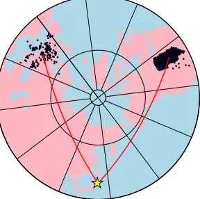
Fig. 3. Selected stations of the USArray and European array are denoted as the blue dots. The JMA hypocenter of the Tohoku-Oki is the yellow asterisk. The red lines are the great circle path from the centroid of each array to the hypocenter. The two arrays are both within 75◦∼90◦from the hypocenter.

A. This curve Bcorresponds to the same location as B but has a delayed absolute source origin time. Curves A and Bsample the same part of the waveform and thus the same amplitude of the signal. Curve Bhas a smaller stack than curve A since it is off phase. Therefore the correct location A is recovered and no artifact is introduced.

(5)

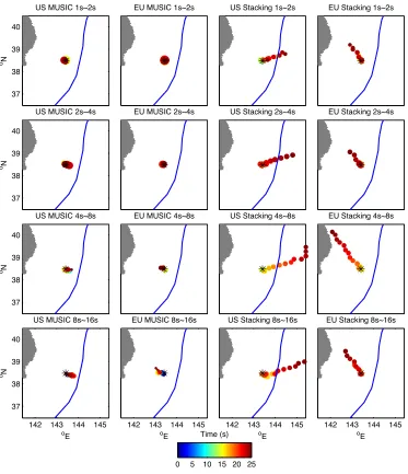
Fig. 4. Back-projection of aftershock synthetics. The synthetic aftershock seismograms at the USArray (left two columns) and European array (right two columns) are processed by the MUSIC and linear stacking techniques separately at periods of 1∼2 s, 2∼4 s, 4∼8 s and 8∼16 s. The location of the aftershock is denoted by the asterisk. The solid circles are the peak of the back-projection images color-coded by time and sized by their relative amplitude with respect to the global maximum. The beamforming results show a “swimming” artifact at all frequencies. The MUSIC estimates are reliable at periods shorter than 4 s. At lower frequencies, the spatial bias is notable but less severe than that of beamforming.

distance thatP-waves travel over the window duration. For the Tohoku-Oki earthquake imaged by the European array and USArray at teleseismic distance, if the trial source region is up to 2 degrees from the epicenter, the standard deviation of the travel time curve is smaller than 1 s, which is a small fraction of the 10 s long window. Hence, the reference window approach is valid in this case.

The reference window approach introduces a time shift, the difference between the mean of B and B, therefore a timing correction is needed (Yao et al., 2011). This cor-rection is readily implemented once the radiator locations have been identiﬁed in each back-projection image frame. The timing shown in our summary maps of HF radiation incorporates this correction, in which the true source time (color coded) of each identiﬁed radiator equals the timing of the back-projection image frame minus the mean of the travel time curve corresponding to the location of the

radi-ator. In the next section, we conduct a series of synthetic tests to compare the frequency domain MUSIC (reference window) and time domain stacking (absolute window).

3. Synthetic Test of Back-Projection at Various

Frequencies

3.1 Point source synthetic test

(6)

up to the teleseismic receivers (Helmberger, 1983). This approach enables incorporating the complexity of regional velocity structures at an affordable computational cost and is ideal for testing teleseismic back-projection techniques at relatively high frequencies. In the SPECFEM3D simu-lation we used a regional tomography model (Miuraet al., 2005) to account for waveform complexity introduced by 3D structures. The synthetic seismograms are computed with a sampling rate of 5 Hz, but, due to the limited com-putation power, accuracy in the SPECFEM simulation is warranted only up to 1 Hz. Future work involves incor-porating realistic small-scale heterogeneities in the velocity model under the receivers to model waveform incoherence and coda decay.

Figure 4 shows the results of MUSIC and time-domain stacking back-projection of the aftershock scenario at vari-ous frequency bands. As expected from the modiﬁed ARF, the peak of the beamforming power progressively migrates along the major axis of the array response. As in our ide-alized ARF analysis, the peak amplitude decreases as it swims. On the other hand, the spatial bias of the MUSIC analysis at high frequencies (0.25 ∼ 1 Hz) is negligible. At frequencies lower than 0.25 Hz, the location shift is no-table but substantially smaller than in time-domain stack-ing. Hence, at low frequency the “swimming” artifact can-not be ignored even with the MUSIC approach.

3.2 Kinematic source synthetic test

To further understand the artifact under more compli-cated and realistic circumstances, we conduct a kinematic rupture scenario involving two branches of simultaneous rupture along a circular rim (Fig. 5). The circle is centered at the hypocenter of theM6.2 aftershock with a radius of 100 km. It is divided into two semicircles by a line trending 210◦through the center. Two simultaneous North-to-South ruptures develop along each semicircle with a rupture speed of 2 km/s. Physically, this scenario is inspired by dynamic simulations in which a rupture front surrounds a circular as-perity, or low-stress region, before breaking it (Dunhamet al., 2003). The ruptures are composed of moving sources with a spatial interval of 40 km. This spacing is chosen so that the sources are dense enough to represent a continu-ous rupture yet the coda wave is still substantial to maintain realistic signal non-stationarity. The Green’s functions are the same as for the M6.2 aftershock. This circular rup-ture model is relatively simple but has enough complexity, including simultaneous sources with a temporally varying spacing.

Figure 5 shows the results of MUSIC and linear beam-forming back-projection of the circular rupture scenario with seismograms computed for both USArray and Euro-pean array at periods from 2 s to 16 s. In order to compare with results by Yaoet al.(2011), we set the time window to be 10 s at the band of 1–4 s and 20 s for 4–16 s. The locations of the ﬁrst and second strongest radiators detected by both arrays in each window are plotted and color-coded by time. The size of the radiators is normalized by the maximum of the beamforming power or MUSIC pseudo-spectrum over the ﬁrst 150 s of the rupture. In the highest frequency band (0.5–1 Hz), the MUSIC result of the Euro-pean array almost exactly reproduces the synthetic rupture

scenario, recovering radiators on the edge of the circle. The USArray result is noisier and distributed within the circle because its Green’s functions have a smaller coherent ar-rival to coda ratio resulting from the nodal orientation of the array with respect to the focal mechanism. In the pe-riod band of 2 s to 4 s, the MUSIC result of both arrays are within the circle. In the low-frequency band (8 s–16 s), the uncertainties become large due to limited resolution and the swimming bias starts to be notable.

In comparison, beamforming is less capable of resolving the simultaneous sources. The recovered radiators are dis-tributed along the expected artifact direction. Here, we also applied a common post-processing technique to weaken the swimming artifact (Koperet al., 2011b). The idea is that although the artifact swims, the true location always has the largest beamformed power. Thus, plotting the high fre-quency power against time and picking only the local max-imum can, in principle, discriminate the true source loca-tion from the spurious sources. The processing is useful when the source process is simple, for instance for a ﬁxed point source or a unilateral rupture, but less effective in complicated rupture scenarios involving multiple simulta-neous sources. In the case of the circular rupture scenario, at relatively short periods (1 s∼4 s) the identiﬁed radiators are located inbetween the true locations. At longer periods (4 s∼16 s) they show considerable bias “downstream” of the true locations along the artifact direction, creating an apparently frequency-dependent rupture pattern.

4. Low-Frequency

Back-Projection

of

the

Tohoku-Oki Earthquake

The along-dip frequency dependent slip migration ob-served in previous back-projection studies is based on the USArray data (Koper et al., 2011a; Mori, 2011; Yao et al., 2011). The other large regional array, the European array, has been processed at high frequency around 1 Hz (Koperet al., 2011b; Menget al., 2011). Analysis of the European array data at longer periods has not been reported before. Here, we back-project the Tohoku-Oki earthquake data recorded by the European array and USArray at pe-riods from 2 s to 16 s with both the MUSIC and linear beamforming methods (Fig. 6). In order to be compa-rable to Yaoet al. (2011), we set the beamforming time window to be 10 s at the band of 1–4 s, and 20 s for 4– 16 s. The locations of the radiators detected by both ar-rays in each frequency band are shown in Fig. 6. The size of the radiators is normalized by the maximum of the beamforming power or MUSIC pseudo-spectrum over the ﬁrst 150 s of the rupture. For time-domain stacking, sim-ilar to the point source synthetic test, we observe a strong swimming effect at periods longer than 2 s. In the highest frequency band (0.5–1 Hz), the artifact is smaller and the beamforming images are roughly consistent with the MU-SIC estimates, which explain the overall agreement of high-frequency back-projection studies.

(7)

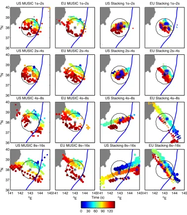
Fig. 5. Back-projection of circular rupture synthetics. The synthetic seismograms of a circular rupture scenario recorded at the USArray (left two columns) and European array (right two columns) are processed by the MUSIC and linear stacking techniques separately at periods of 1∼2 s, 2∼4 s, 4∼8 s and 8∼16 s. The location of the aftershock is denoted by the black asterisk. The black circle is the hypothetical circular path of the rupture scenario. The solid circles are the peak of the back projection images color-coded by time and sized by their relative amplitude with respect to the global maximum. The blue asterisks are the “temporal local maximums” of the stacking result. The MUSIC recovers the rupture reasonably well at high frequency but loses the resolution beyond 4 s. The time-domain stacking method shows a bias resulting from the swimming artifact.

bands at both arrays, except in the 8∼16 s band which shows linear patterns corresponding to the artifact. We therefore restrict analysis of frequency-dependent source behavior based on MUSIC results to the band of 1∼8 s. As shown by the synthetic tests, even with the reference win-dow strategy and the MUSIC method, the artifact at lower frequency is signiﬁcant. For a given period, the radiators imaged by MUSIC with the European array are always to the west of those imaged with the USArray. At the USAr-ray, an eastward migration of about 70 km is seen between 1 and 8 s. This is consistent with the most clearly-reported frequency-dependent shifts by compressive sensing (Yao

et al., 2011). However, this trend is absent in the Euro-pean array results, which do not show a notable frequency-dependent variation. This difference is consistent with the stronger artifact in the USArray, as shown in Fig. 5, due

to the smaller signal to coda ratio resulting from its nodal orientation. Therefore, a frequency-dependent source lo-cation is not needed to explain the observations within the 1∼8 s band. This indicates that any true frequency depen-dent source migration is minor compared to the 70 km shift apparent in the USArray back-projection.

5. Summary and Discussion

(8)

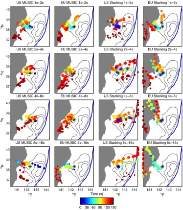
Fig. 6. Back-projection of the Tohoku-Oki earthquake at various periods (1 s∼16 s) of the USArray and European array data with the linear stacking and MUSIC approaches. The hypocenter is denoted by the black asterisk. The location of the radiators are colored by time and sized by the amplitude with respect to the maximum. The blue asterisks are the “temporal local maxima” of the stacking result. The background grey lines are 12 m, 14 m and 36 m slip contours of a geodetic and seismic joint inversion model (Weiet al., 2012). The beamforming results are dominated by the artifact at periods longer than 4 s. The MUSIC results are consistent over all frequency bands. Minor up-dip migration shows up in the period of 1 s∼8 s at the USArray, but is within the range expected from the “swimming” artifact and is absent in the European network.

to migrate towards the trench at increasing periods within the period band of 1∼8 s. An alternative interpretation is that the most substantial transition from deep to shallow slip occurs at periods longer than 16 s, which implies an even longer rise time in the shallow portion of the megath-rust. Furthermore, given that the swimming artifact is sub-stantial in the time-domain stacking back-projections espe-cially at long periods, and that this bias at the USArray be-haves similarly to the potential frequency-dependent along-dip migration of slip, we consider that further tests and val-idations need to be performed before one can conclude that the along-dip slip migration can be observed by the low fre-quency back projection.

Our study also poses an interesting question: over which frequency band can we reliably image earthquake rupture processes by teleseismic back-projection? To image the

2011 Tohoku-Oki earthquake by the time-domain stacking technique with the USArray and European array, we deter-mined that the frequency should be above 0.25 Hz to avoid substantial artifacts. As for the MUSIC technique, which suffers less severely from the swimming artifact, we sug-gest that the low-frequency results around 0.1 Hz can indi-cate ﬁrst-order spatial patterns, but the ﬁner details of the images are not reliable due to the limited resolution.

(9)

simultaneous sources.

One mystery that remains to be explained is the discrep-ancy between the MUSIC and compressive sensing result (Yaoet al., 2011). In principle, they are both performed in the frequency domain and share the reference window strat-egy, therefore both should suffer less from the swimming artifact. Yet, compressive sensing provide a large trench-ward shift at 10 s∼20 s, which is absent in the 8 s∼16 s band result with MUSIC. Efforts could be devoted to under-stand the other potential bias and artifact of various back-projection techniques. This concern also demonstrates the need to perform more rigorous synthetic tests involving more realistic rupture scenarios and crustal velocity mod-els, which we will address in future work.

Acknowledgments. This research was supported by NSF grant EAR-1015704, by the Gordon and Betty Moore Foundation and by the Southern California Earthquake Center, which is funded by NSF Cooperative Agreement EAR-0106924 and USGS Coopera-tive Agreement 02HQAG0008. The EarthScope USArray and the European ORFEUS data center were used to access the data. This paper is Caltech Tectonics Observatory contribution #198 and Cal-tech Seismolab contribution #10075.

References

Asano, K. and T. Iwata, Strong Ground Motion Generation during the 2011 Tohoku-Oki Earthquake,AGU abstract, U42A-03, 2011.

Dunham, E. M., P. Favreau, and J. M. Carlson, A supershear transition mechanism for cracks, Science, 299(5612), 1557–1559, doi:10.1126/science.1080650, 2003.

Helmberger, D. V., Theory and application of synthetic seismograms, in Earthquakes: Observation, Theory and Interpretation,Soc. Ital. di Fis., Bolgna, Italy, 174–222, 1983.

Huang, Y., L. Meng, and J.-P. Ampuero, A dynamic model of the frequency-dependent rupture process of the 2011 Tohoku-Oki earth-quake,Earth Planets Space,64, this issue, 1061–1066, 2012. Ishii, M., High-frequency rupture properties of theMw 9.0 off the

Pa-ciﬁc coast of Tohoku Earthquake,Earth Planets Space,63(7), 609–614, doi:10.5047/eps.2011.07.009, 2011.

Ishii, M., P. M. Shearer, H. Houston, and J. E. Vidale, Teleseismic P wave imaging of the 26 December 2004 Sumatra-Andaman and 28 March 2005 Sumatra earthquake ruptures using the Hi-net array,J. Geophys. Res.—Solid Earth,112(B11), doi:10.1029/2006jb004700, 2007. Kato, N., How frictional properties lead to either rupture-front focusing or

cracklike behavior,Bull. Seismol. Soc. Am.,97, 2182–2189, 2007. Koketsu, K. et al., A uniﬁed source model for the 2011

To-hoku earthquake, Earth Planet. Sci. Lett., 310(3–4), 480–487, doi:10.1016/j.epsl.2011.09.009, 2011.

Koper, K. D., A. R. Hutko, and T. Lay, Along-dip variation of teleseis-mic short-period radiation from the 11 March 2011 Tohoku earthquake (M(w) 9.0),Geophys. Res. Lett.,38, doi:10.1029/2011gl049689, 2011a. Koper, K. D., A. R. Hutko, T. Lay, C. J. Ammon, and H. Kanamori, Frequency-dependent rupture process of the 2011 Mw 9.0 Tohoku Earthquake: comparison of short-periodPwave backprojection images and broadband seismic rupture models,Earth Planets Space,63(7), 599–602, doi:10.5047/eps.2011.05.026, 2011, 2011b.

Lay, T., H. Kanamori, C. J. Ammon, K. D. Koper, A. R. Hutko, L. Ye, H. Yue, and T. M. Rushing, Depth-varying rupture properties of subduction zone megathrust faults,J. Geophys. Res.,117, B04311, doi:10.1029/2011JB009133, 2012.

Lee, S. J., B. S. Huang, M. Ando, H. C. Chiu, and J. H. Wang, Evidence of large scale repeating slip during the 2011 Tohoku-Oki earthquake,

Geophys. Res. Lett.,38, doi:10.1029/2011gl049580, 2011.

Meng, L. S., A. Inbal, and J. P. Ampuero, A window into the complexity

of the dynamic rupture of the 2011 Mw 9 Tohoku-Oki earthquake,

Geophys. Res. Lett.,38, L00g07, doi:10.1029/2011gl048118, 2011. Miura, S., N. Takahashi, A. Nakanishi, T. Tsuru, S. Kodaira, and Y.

Kaneda, Structural characteristics off Miyagi forearc region, the Japan Trench seismogenic zone, deduced from a wide-angle reﬂection and re-fraction study,Tectonophysics,407, 165–188, 2005.

Miyake, H., Y. Yokota, H. Si, and K. Koketsu, Earthquake Scenarios Generating Extreme Ground Motions: Application to the 2011 Tohoku Earthquake,AGU abstract, S 52B-07, 2011.

Mori, J., The Great 2011 Tohoku, Japan Earthquake (Mw9.0): An Unex-pected Event, Southern California Earthquake Center Annual Meeting, Special Invited Talk, 2011.

Nakahara, H., Seismogram envelope inversion for high-frequency seismic energy radiation from moderate-to-large earthquakes,Adv. Geophys., 50, 401–426, doi:10.1016/S0065- 2687(08)00015-0, 2008.

Rost, S. and C. Thomas, Array seismology: Methods and applications,Rev. Geophys.,40(3), doi:10.1029/2000rg000100, 2002.

Roten, D., H. Miyake, and K. Koketsu, A Rayleigh wave back-projection method applied to the 2011 Tohoku earthquake,Geophys. Res. Lett., doi:10.1029/2011GL050183, 2011.

Sato, H. and M. C. Fehler,Seismic Wave Propagation and Scattering in the Heterogeneous Earth, Springer-Verlag and American Institute of Physics Press, 1998.

Sato, M., T. Ishikawa, N. Ujihara, S. Yoshida, M. Fujita, M. Mochizuki, and A. Asada, Displacement above the hypocenter of the 2011 Tohoku-Oki Earthquake, Science, 332(6036), 1395–1395, doi:10.1126/science.1207401, 2011.

Shao, G., X. Li, C. Ji, and T. Maeda, Focal mechanism and slip history of the 2011 Mw 9.1 off the Paciﬁc coast of Tohoku Earthquake, con-strained with teleseismic body and surface waves,Earth Planets Space, 63(7), 559–564, doi:10.5047/eps.2011.06.028, 2011.

Simons, M.et al., The 2011 magnitude 9.0 Tohoku-Oki Earthquake: Mo-saicking the megathrust from seconds to centuries,Science,332(6036), 1421–1425, doi:10.1126/Science.1206731, 2011.

Tromp, J., D. Komatitsch, and Q. Y. Liu, Spectral-element and adjoint methods in seismology,Commun. Comput. Phys.,3(1), 1–32, 2008. Walker, K. T. and P. Shearer, Illuminating the near-sonic rupture velocities

of the intracontinental Kokoxili Mw 7.8 and Denali Mw 7.9 strike-slip earthquakes with global P-wave back projection imaging,J. Geophys. Res.,114, doi:10.1029/2008JB005738, 2009.

Wang, D. and J. Mori, Rupture process of the 2011 off the Pa-ciﬁc coast of Tohoku Earthquake (Mw 9.0) as imaged with back-projection of teleseismicP-waves,Earth Planets Space,63(7), 603– 607, doi:10.5047/eps.2011.05.029, 2011.

Wei, S., R. Graves, D. Helmberger, J.-P. Avouac, and J. L. Jiang, Sources of shaking and ﬂooding during the Tohoku-Oki earthquake: A mixture of rupture styles,Earth Planet. Sci. Lett., doi:10.1016/j.epsl.2012.04.006, 2012.

Xu, Y., K. D. Koper, O. Sufri, and L. Zhu, Rupture imaging of the Mw 7.9 12 May 2008 Wenchuan earthquake from back projection of teleseismic P waves, Geochem. Geophys. Geosyst., 10, Q04006, Doi:10.1029/2008GC002335, 2009.

Yao, H. J., P. Gerstoft, P. M. Shearer, and C. Mecklenbrauker, Compressive sensing of the Tohoku-Oki Mw 9.0 earthquake: Frequency-dependent rupture modes,Geophys. Res. Lett., 38, doi:10.1029/2011gl049223, 2011.

Yao, H. J., P. Shearer, and P. Gerstoft, Subevent location and rupture imaging using iterative backprojection for the 2011 Tohoku Mw 9.0 earthquake,Geophys. J. Int., 2012 (submitted).

Yue, H. and T. Lay, Inversion of high-rate (1 sps) GPS data for rupture process of the 11 March 2011 Tohoku earthquake (M(w) 9.1),Geophys. Res. Lett.,38, doi:10.1029/2011gl048700, 2011.

Zerva, A. and V. Zervas, Spatial variation of seismic ground motions,Appl. Mech. Rev.,55(3), 271–297, 2002.