Earth Planets Space,51, 525–541, 1999
The dynamical parameters of turbulence theory as they apply to middle
atmosphere studies
W. K. Hocking
The University of Western Ontario, London, Ont., Canada
(Received August 21, 1998; Revised January 20, 1999; Accepted April 12, 1999)
The study of turbulent heating and diffusion in the middle atmosphere is complicated by some subtle points relating to the application of existing theory. Incorrect interpretation of turbulent spectra can result, leading to errors in estimates of the strengths of turbulence by factors of 5 and more. In this short review, the relevant turbulent spectra and equations are considered, and their applications in middle atmosphere studies are outlined. New developments with regard to some of this theory, and especially new understandings about the dynamical parameters used in some of these applications (often referred to as the “constants” of the equations) are described. Current areas of uncertainty are also considered, both in relation to turbulent energy dissipation as well as diffusion over various scales.
1.
Introduction
In studies of turbulence, the optimum spectra to use for calculations of kinetic energy dissipation rates are often the velocity spectra. These are dealt with in some detail in the literature (e.g. Batchelor, 1953; Tatarskii, 1961, 1971). For freely decaying turbulence we can consider ε, the kinetic energy dissipation rate, as
ε= −d
dt
1 2
u2+v2+w2, (1)
whereu2+v2+w2is the total mean square velocity fluc-tuation, and12u2+v2+w2is therefore the mean kinetic energy per unit mass at any instant in time (Batchelor, 1953, page 86). The overbar refers to a spatial average. (An even more fundamental discussion about the energy dissipation rate can be found in Batchelor, 1967, Subsection 3.4, but that is beyond our requirements for this paper.)
If an experimentalist can obtain velocity fluctuations at scales within the inertial range of turbulence, or even into the viscous range, then calculation of kinetic energy dissipation rates is very straight forward. For example, if an observer is dealing with isotropic, homogeneous turbulence, and if that observer can make measurements at scales within the inertial range and deep into the viscous range, then the kinetic energy dissipation rateεcan be found directly by integrating across the spectrum as
ε=2 ∞
0
νk2E(k) (2)
whereν is the kinematic molecular viscosity coefficient, k
is the wave number, andE(k)is the spectral density of ve-locity fluctuations (sum of all three components) over a shell
Copy right cThe Society of Geomagnetism and Earth, Planetary and Space Sciences (SGEPSS); The Seismological Society of Japan; The Volcanological Society of Japan; The Geodetic Society of Japan; The Japanese Society for Planetary Sciences.
in wave-number space of radiusk(e.g. see Batchelor, 1953; Hocking and Hamza, 1997, and references therein). How-ever, in atmospheric sciences, determination ofE(k)down to scales this small is rarely possible. In the middle atmosphere, it simply cannot be achieved with current technology.
If it is possible to determine velocity fluctuations down to scales at least into the inertial range, determination ofεis still modestly easy, although one often needs to make assump-tions about the form of turbulence (isotropic, Kolmogoroff theory etc.). Examples of such applications exist in the lit-erature: for example, Barat (1982) has shown how this may be done using structure functions.
However, Barat’s measurements required a high altitude balloon, and special instrumentation. Measurements into the upper middle atmosphere by this method are limited by a ceiling on the balloon altitude. In-situ measurements above say 40 km altitude are limited to rockets, and because these must travel at high speed, they cannot sample the velocities with sufficient resolution to apply such methods.
Measurements of middle atmosphere turbulence are there-fore largely limited to radar techniques, and occasional rocket and balloon studies. Within these categories, only special balloon-borne instrumentation is capable of direct velocity measurements at sufficient spatial and temporal resolution to enable direct calculation ofε, and even then high altitude balloons are only flown rarely. All other methods involve measurements of velocity fluctuations which effectively in-tegrate over moderately large intervals of scale, or involve measurements of parameters other than the velocity fluctu-ations. In the former case, the integration limits and instru-mental weighting are often hard to determine, and in the latter case it is often necessary to make various assumptions, and determine other parameters such as background gradients, before turbulence strengths can be calculated.
This review focuses on a critical examination of the as-sumptions made in developing the formulae which are used in determination of middle atmosphere turbulence strengths,
and highlights recent developments in this area.
2.
Currently Used Formulae
The following equations present various formulae which are currently used for determinations of middle atmosphere turbulence strengths.
Variations of these formulae have been presented by, for example, Weinstock, (1978a,b, 1981), and Hocking (1983, 1986). The term ωB is the V¨ais¨al¨a-Brunt frequency, ε is the kinetic energy dissipation rate,σrefers to a typical root-mean-square velocity (to be specified in more detail later), andLBis a scale related to the larger eddies.
These equations appear deceptively simple, but they are in fact complicated by several factors. Principal amongst these is the fact that the termσ2 is sometimes ill-defined.
The constantsc0andc1are critically dependent on howσ2
is determined. Formulae of this type are often used in both in-situ and radar studies, but the nature of the determination of σ2 must be very carefully considered. For example, in radar studies it is usually an integral over the radar volume, and over the duration of the radar record used for the cal-culation. The details of this integration process need to be carefully considered. As we will see, there are also addi-tional complications, and even the choice of the scaleLBis
complicated.
In fact there are some references which use yet another variant on Eq. (3). This equation takes the form
ε=c6(σ2)3/2/Lr (6)
whereLris a scale associated with the radar beam and
pulse-length, and not the scaleLBdefined above (e.g. Labitt, 1979; Bohne, 1982; Doviak and Zrnic, 1984). We therefore need to ask: which of these two options (i.e. Eqs. (3) or (6)) is preferable?
Thus we recognize that these equations, despite a decep-tively simple appearance, are not well understood, and we pose the questions: What do we mean byσ2? Which scale “L”should we use? Answering these questions will be one of our responsibilities in this paper.
There are also other equations which appear in the litera-ture which need to be more properly understood. Some such equations are the expressions
Again, these are very simple equations, but with hidden complications. We will define the various terms and consider these expressions shortly.
Another expression used in the literature to determineε, which utilizes the mean square refractive index fluctuation quantityC2
nis often called the“potential refractive index structure constant”, although the use of the word“constant”here can be quite misleading, since the quantity is far from constant— it in fact varies markedly as a function of the intensity of the turbulence. Nevertheless, we must persist with this usage, since it is very common. However, the reader should bear in mind thatC2
nis in fact a measure of the amount of refractive index fluctuation in a given turbulent patch, and is not to be considered in the same category as the other dynamical parameters (also referred to as “constants”) which are the topic of this paper. Again, the above expression looks simple enough, but application of this expression is complicated by determination of the term“F”(which represents the fraction of the radar volume which is turbulent), and by a proper determination of the“constant”γ—which in fact turns out to be Richardson-number dependent. We will not consider the factor“F”any further here; our main interest is in the parameterγ. Discussions relating to“F”can be found in Van Zandtet al.(1978, 1981) and Hocking and Mu (1997). Finally, there is another expression which appears to be exquisitly simple, yet hides a multitude of complexity. This is the expression
K =c2 ε
ω2 B
(11)
where K represents a diffusion coefficient. This relation purports to relate the rates of atmospheric diffusion and the value of the kinetic energy dissipation rate. However, it raises many issues. It may be derived from modestly simple argu-ments; for example, Fukaoet al.(1994), Appendix A, gives one example. However, there are yet further questions about this. Is the derivation too simplistic? Is it valid at all? If it is valid, what should be the“constant”c2? Different authors have proposed different values forc2. If indeed it does ap-ply, is it valid over all scales? If the scale-range is limited, what limits exist? McIntyre (1989) has even considered that the value ofc2 might depend in some way on the mode of
turbulence generation, and the degree of super-saturation of the waves which generate the turbulence. How realistic is this proposal? In that case, it would not even make sense to assume thatc2is a constant for an individual event, although
there might still be some long-term average value ofc2which can be applied to the middle atmosphere. We cannot address all these issues, but will try and consider at least some of them.
Thus, while we recognize that these formulae are used in the literature for determination ofεandK, we also recognize that each equation embodies a complication of one sort or another. A major objective of this paper will be to highlight, and where possible clarify, these complications.
W. K. HOCKING: DYNAMICAL PARAMETERS OF TURBULENCE 527
to simply be a summary of the main and simplest tools used in turbulence studies. We begin with functions associated with measurements of velocity, and later move to measurements of tracers and scalars.
In our next sections, we then begin to address some of the questions raised above.
3.
Turbulence Scales and Inverse Scales
Wefirst turn to a discussion of the Eqs. (7) to (9), mainly because the questions posed in relation to these expressions are some of the simplest to answer.
Thefirst equation, (7), is a derivation produced from di-mensional analysis. However, once derived it can be usefully employed as a scaling length. Physically, it is a scale within the viscous range of the turbulence, and represents a typical scale at which energy transfer by scale-cascade, and energy dissipation to heat, are comparable. The scale0 is a scale which represents the transition between the inertial and vis-cous ranges of turbulence, and is defined in terms of the in-tercept between extrapolations of the spectral forms in these two ranges (e.g. see Tatarskii, 1971). It is always bigger than
η, and the constantc4is in fact fairly well known. However, it is important to recognize that evenc4depends on whether one is using measurements of velocityfluctuations or some sort of constituent or tracer. Typical values ofc4are 7.4 for temperaturefluctuations (e.g. Hill and Clifford, 1978), and
(15C)3/4(whereC =2.0), or 12.8, for velocityfluctuations
(e.g. Tatarskii, 1961).
Thus these scales are at least fairly well understood, al-though on occasions some authors have assigned them to have units ofmetres per radian, which is wrong. They are simply units of length.
Equation (9) does introduce some extra complications, however, which sometimes lead to confusion. The scaleL0
is a vertical scale at which the RMSfluctuations due to the turbulence are equal to the change in the mean value of the same quantity over the same vertical scale. This is quite dif-ferent toLB, which is a scale at the“large-scale end”of the
inertial range of the spectrum. The latter quantity is usually much larger than thefirst—often by more than an order of magnitude (e.g. see Hocking, 1985, who gives a ratio in the order of 30).
To complicate things further, an alternative scale toLBis
often used, which equalsε1/2ω−3/2
B and is called the Ozmidov
scale. This differs fromLBonly by a multiplicative constant
of 2π/c3, so conceptually is very similar to LB. We will
generally use LB, since this has become more common in middle atmosphere work, and Barat (1982) has shown that it does indeed seem to relate fairly nicely to the low wave-number end of the inertial range.
Another common problem which occurs in discussions about the scales of turbulence is the use of inverse scaling factors. Whilst a scale is assigned a“wavelength”λ, and its corresponding wavenumber isk = 2π/λ, it is not uncom-mon to use special inverse scales which relate to particular spatial lengths by a simple reciprocal relation. For example, sometimes a scalekB∗ =1/LBis used for scaling purposes.
This seems at odds with the wavenumberkB=2π/LB, but in
fact there is no conflict; we will therefore dispense with this issue here. LBis a“typical”scale, but does not particularly
represent the distance between the maxima of any special si-nusoidalfluctuation. Therefore there is no obligation to use 2πas the scaling constant, sok∗B=1/LBis just as useful for
scaling purposes as 2π/LB. Problems arise, however, when kB∗ is referred to as a “wavenumber”; it is in fact not one, and should be considered (when used) as nothing more than an inverse scaling factor. Confusion arises because scaling parameters like this are sometimes referred to as “wavenum-bers”, and because they are often denoted by symbols which are traditionally used for harmonic quantities. If, on the other hand, one is talking of true wavenumbers, and their relation to“wavelengths”, then one must usek=2π/λ.
4.
Relation between
εεεεεεεεand
σσσσσσσσ22222222In this section, we wish to address the issue of the cor-rect relation betweenσ2andε, as described in Eqs. (3) and (6). The equations look similar, but in fact are very different conceptually, and we need to understand why.
In studies of turbulence with a radar, one usually mea-sures a complex-amplitude time-series which is a result of radio-wave scatter from a region of space called the“radar volume”. This volume is defined by the radar beam and radar pulse-length. Within this volume, scatterers are mov-ing with a variety of velocities, and the observed signal is due to a combination of Doppler shifted echoes produced when the radiowaves scatter from these entities. The received sig-nal can be Fourier transformed to produce a spectrum, which has a half-power half-width of f1/2, and an associated
vari-ance fv2. If we multiply fv2by(λ/2)2, whereλis the radar wavelength, then we produce a variance in terms of velocity units, which we denote asσ2. This variance is an integrated effect of all the velocityfluctuations within the radar volume, as shown diagrammatically by Hocking (1983).
Detailed derivations of the relation between the turbulence velocity spectrum (which describes the fluctuations inside the radar volume) and the value ofσ2have been presented
by (amongst others) Hocking (1983), Labitt (1979), Bohne (1982) and Hocking (1996a). In the following subsections, we will briefly re-visit some of these derivations.
To begin, we will follow the derivation presented by Hocking (1983), which produces Eq. (3).
4.1 Buoyancy scale dependence betweenσσσσσσσσ22222222andεεεεεεεε
Assuming a Kolmogoroff form for the turbulence spec-trum, Hocking (1983, 1986) has shown that
σ2∝
k=4π/λ
2π/LB
ε2/3k−5/3dk, (12)
whereσ is the root mean square velocity deduced from the spectral width of the signal. At this stage we will not concern ourselves with the constants of proportionality; our main interest here is in the general form of the equation. We will shortly produce a more sophisticated form of this equation in which the relevant constants of proportionality will become clearer. This equation expresses the fact that the velocity variance measured by the radar is the integrated effect of different scales within the radar volume.
Upon integration we obtain the following expression:
Assuming thatLBλ/2 we have the following
relation-The value ofc1differs somewhat for different assumptions about the constants involved in the Kolmogoroff spectrum, but Hocking (1983) has given a value of c1 of 3.5. This value assumes that thefluctuations producing the radar signal are produced in roughly equal proportion by scales in the buoyancy range and the inertial range. We shall re-address this assumption shortly.
If, in addition, we use the relation between the buoyancy scaleLBand the V¨ais¨al¨a-Brunt frequency which was
speci-fied earlier as
(Weinstock, 1978b), we may then write
ε=c0σ2ωB (16)
wherec0is a constant (∼0.45).
In contrast to this expression, (which is commonly used in mesospheric and stratospheric radar studies), equations relating radar spectral widths and turbulent energy dissipa-tion rates which have been presented in the meteorological literature have tended to ignore the possibility that the buoy-ancy scale may play a role in the relation betweenεandσ2.
Rather, they have assumed that either the length of the radar pulse, or the radar beam-width, (whichever is larger) is the most important parameter in determining thisε—σ2relation.
We will now look at this particular derivation in more detail.
4.2 Radar volume dependence betweenσσσσσσσσ22222222andεεεεεεεε
The following derivation briefly summarizes that pre-sented by Labitt (1979), and also prepre-sented by Hocking (1996a). We do not intend to repeat their derivations in detail here, and so we start with the relation
σ2= which is derived in those references.i jis described in Eq. (B.4), and in this case we takei = ji.e. both velocity com-ponents aligned in the direction parallel to the direction of traverse (in this case the direction of traverse of the radar beam) through the patch of turbulence (see Appendices A to D). The term in square brackets is simply 1 minus the Fourier transform of the radar volume, and therefore takes into ac-count the radar weighting. Equation (17) is in fact similar in some aspects to Eq. (12), but there are also some impor-tant differences between the two. The former one essentially assumes that all radial motions are parallel to the bore-sight direction of the radar, while this newer one recognizes that there may be contributions from off-bore-sight components if the beam is broad. Equation (12) also contains no specific radar weighting, but does contain a lower limit onkwhich is defined by the largest turbulence scales. Equation (17) con-tains no such turbulence-defined limit, and this will shortly prove to be an important point.
It is also important to point out that neither of these for-mulae recognize the fact that the velocity spectrum should actually be anisotropic at scales comparable to and larger
than LB. However, since for MST work the radars usually
point vertically, and it is primarily the vertical velocity spec-trum which affects the spectral width, it is only necessary that a reasonable estimate of the vertical velocity spectrum is produced for our work here. In this case, we specifyE(k), and the vertical velocity spectrum is derived from that, but we have allowed a reasonable range of possibilities forE(k), and therefore a reasonable range of vertical velocity spec-tra. The key point is thatE(k)is chosen so that thevertical velocity spectra are realistic. Since horizontalfluctuations are of secondary significance for a vertically pointed, narrow beam, the issue of anisotropy is not so crucial here. Hocking (1996a), and Hocking and Hamza (1997) has discussed the issues of anisotropy in a little more detail.
If one then takes the classical inertial range spectrum (e.g. see Tatarskii, 1971), then the spectrum of vertical velocities as a function of wave numberkis
(k)= E(k)
wherekis the magnitude ofkand so is a scalar satisfying
k2=k2
x+k2y+k2z,E(k)=αε2/3k−5/3, andαis a numerical constant with value 0.7655C, whereC =2.0 (see Eq. (B.4)). The following expression for the velocity variance mea-sured by the radar may now be obtained:
σ2=1
Finally, the following expressions forϒare valid: Firstly ifa ≥b:
Where Fis the confluent hypergeometric function. To a good approximation we can write
ε=0.79σ
3
Lr
.cc (24)
whereLris the largest of the pulse length and the beam width,
andccis a correction factor very close to 1.
As noted, Eqs. (14) and (24) are conceptually very differ-ent. Why should this be?
W. K. HOCKING: DYNAMICAL PARAMETERS OF TURBULENCE 529
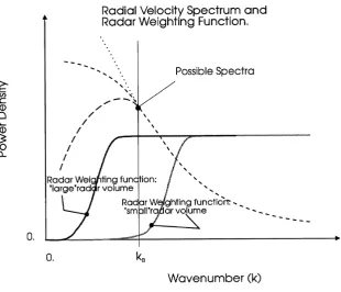
Fig. 1. Graphs showing the radial velocity spectra and radar weighting functions for different assumed spectra and radar volumes.
the spectrum may have a“roll-over”at small wavenumbers, where a“roll-over”refers to a moderately abrupt but smooth change in slope. This may be evident as a“knee” in the spectrum, or even a local peak. Whether such a“rollover” exists depends on what one assumes about the nature of the low wave number spectrum (often the gravity wave spec-trum) at the scales close to the turbulence regime. It also depends on which radial velocities are being measured—a vertically pointed radar measures principally the vertical fluc-tuating motions, whilst a horizontally pointed radar measures largely horizontal components of motion. In our discussion we are primarily considering near-vertical beams, which are the main modes used for middle atmosphere studies.
This“roll-over”is what causes the Labitt formalism to break down. Labitt assumed that the Kolmogoroff spectral form (i.e.∝ k−5/3) continued down tok = 0, and this is
why his integral involves Lr. Such an assumption may be valid if the radar is used to point its beam horizontally (as is the case, for example, with the meteorological NEXRAD radars). However, if this“roll-over point”in the spectrum occurs at wave-numbers which are greater than the lowest wave-numbers corresponding to the radar volume, then the integral begins to involveLB. For most middle atmosphere radars, near-vertical beams are used, so this latter possibility is likely.
Figure 1 shows how this comes about. The integrand in-volves a product of the spectrum and the weighting function, and it is seen that if the weighting function is that for a“small” radar volume, and we follow it from largekback to smallk, then the weighting drops to zero beforekB is encountered.
Thus the integral does not involve any portion of the spectrum atk values belowkB. However, in the case labelled“large
radar volume”, the radar weighting function does not start to approach zero (reading from the right) until the spectrum has entered the“buoyancy”regime. Thus the nature of the spectrum in this low wave-number end begins to affect the integral.
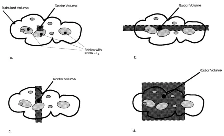
The situation is also indicated diagrammatically, but in a different way, in Fig. 2. In thefirst case, we show a region of turbulence with the radar volume being substantially smaller than the largest scales of turbulence. In this case, we expect the Labitt formula to apply. However, the other diagrams (b, c, and d) show cases where some part of the radar volume exceeds (or is at least comparable with) the largest scales of the turbulence. In this case, we expect the formula with an
LBdependence to apply.
Thus Labitt has ignored the small wavenumber depar-ture from the inertial range law. However, we should also point out that Eq. (12) is also only a crude approximation, since it assumes that the spectrum drops abruptly to zero at the wavenumberkB. Therefore both approaches have their weaknesses—Eq. (12) is mathematically crude, while Eq. (17) is mathematically rigorous but ignores the true small-wavenumber spectral variation. It makes sense to combine the formalisms, to try and take advantage of both of their strengths.
In the following section, we will put the concepts dis-cussed above into a mathematical setting, and demonstrate that our expectations are valid. In fact, we will show that the largest cross-volume length of the radar volume must be less than one half of the buoyancy scale for the Labitt formula to apply—in all other cases, the formula involvingLBis more
Fig. 2. Different possible relations between the radar volume and a patch of turbulence. Only in thefirst case is the behaviour of the turbulence spectrum at smallk(i.e. belowkB) unimportant in determing the relation betweenεandσ. In all other cases, the relation betweenεandσhas akBdependence.
5.
Combining the Buoyancy Part of the Spectrum
within the Labitt-Formalism
We will now re-address Eqs. (17) and (18), but this time we will permitE(k)to have a“roll-over”point at low wave-number. We will see that this substantially changes Eq. (24), and in fact makes the result appear more like (14) in many cases.
To begin, we propose the following possible shape of the spectrum at smallk, (as discussed by Hocking, 1996a):
E(k)=αε2/3 k −5/3
[1+χk(k/kB)n]
(25)
wherekB=2π/LBand where the value ofndetermines the
form of the low wave-number part of the spectrum. The value ofχk affects the relative positions of the low-wavenumber “roll-over point” in the spectrum and the quantity kB.
Hocking (1996a), used the special casesn = −3 and−4/3, because they represent extreme examples of the possible spectral forms, and thus set reasonable limits on our for-mulae. They correspond to cases with E(k)∝ k+4/3 and k−1/3at smallkrespectively. Examples are shown
diagram-matically in Fig. 3 for the case of χk = 1.0. Clearly the “knee”(or“peak”for the casen= −3) is close to the value ofkB, so henceforth we will useχk=1.0 as a reasonable ap-proximation, although we recognize that future more detailed experimental studies might give slightly different values for this parameter. At present, however, there are insufficient experimental data to better defineχk.
As noted prior to Eq. (18), this equation implicitly assumes an isotropic spectrum. However, this is not entirely unrea-sonable for the cases we wish to consider. In addition, for a vertically directed beam it is principally the vertical velocity
Fig. 3. Representative forms for the turbulence spectrumE(k), including typical possible variations at smallk. Specifically these graphs show Eq. (25), forn= −3 and−4/3. Then= −3 case corresponds to a power law of the typek4/3at smallk, and is represented by the broken line; the
n= −4/3 case corresponds to a power law of the typek−1/3at small
k, and is represented by the solid line. In both cases the buoyancy scale is the same and equals 250 m; the corresponding wavenumber lies very close to the peak in the broken curve (from Hocking, 1996a).
fluctuations which are important, so as long asE(k)is cho-sen so as to produce a reasonable vertical velocity spectrum, any lack of isotropy is not too critical to our arguments. It should also be recognized that we only seek to place rea-sonable limits on the relation between spectral widths and the energy dissipation rates, so great accuracy in specifying
W. K. HOCKING: DYNAMICAL PARAMETERS OF TURBULENCE 531
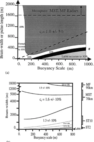
Fig. 4. These two graphs show corrections to the formulaε(0.45σ2ω
B)in radar applications. Specifically, they show values forcfin the expression ε(0.45σ2ω
B)c−f2/3, for cases of (a)n= −3 and (b)n= −4/3. Cases where the“Labitt formalism”should be used are also indicated. In case (b), the scale on the right side indicates the approximate heights at which the appropriate beam-widths shown on the left apply, assuming an angular beam-width of typically 2 to 5 degrees.
as an experimentally measured quantity, which is another reason why we have taken this more approximate course of action.
We now must determine
ϒ =
π
θ=0
∞
k=0
sin3θ k
−5/3
[1+(k/kB)n]
×[1−e−k2[a2sin2θ+b2cos2θ]]dkdθ. (26)
Hocking (1996a) has numerically integrated this expres-sion for a wide range of combinations ofkBand pulse length.
With respect to the casen = −3 (E ∝ k4/3at smallk), he
found the following. Provided that the larger of the radar pulse-length and beam-width exceeds one half of the
buoy-ancy scale, then to very good accuracy,ϒcan be represented closely by the following expression:
ϒ=(0.45LB)2/3. (27)
Hence, using Eq. (21) we obtain the relation
ε=3.3σ
3
LB =0.47σ
2ωB. (28)
This compares very favourably to the estimates made in the earlier literature, in which the equation ε = 0.45σ2ω2 B
has been given e.g. see Eq. (16). Figure 4(a) shows a contour graph in which a measure of the ratio of the true value of
widths and various buoyancy scalesLB. The area in which
the Labitt formula is accurate is also highlighted; note that throughout most of the region described by this graph the dependence ofεonLBis very important and the Labitt
for-malism is generally not valid. As experimental support for this prediction, it is noteworthy that Bohne (1981: abstract), who attempted to use the Labitt formalism to produce radar measurements ofε, and then compared them with measure-ments made in-situ, found that he could only make useful estimates ofεfor those cases in which the radar pulse length was less than one half of the buoyancy scale. The reason for the inaccuracy of the radar measurement in these cases of smallLBwas almost certainly because Eq. (28) should have been used, rather than the Labitt approach.
Let us now turn to the case ofn = −4/3. In this case the spectrum goes ask−1/3asktends to 0. Then in fact numerical
integration of Eq. (26) over a wide range of possible buoyancy scales and possible pulse lengths and beam widths gives the following expression:
wherecfis a correction factor. Even in this case, where the
buoyancy range runs somewhat smoothly into the inertial range, but where the energy involved in the buoyancy range is higher than that in the inertial range, it can be seen that the dependence onLBis still significant and the expression given by Labitt is generally not appropriate.
Figure 4(b) shows the value of the correction factor over a wide range of beam widths and buoyancy scales. Note that the region in which the Labitt formalism is approximately correct is indicated and is clearly only a small portion of the region. For MST radars the Labitt equation is almost never valid and the previous expression (29) is correct. Further-more, the correction factor is a fairly slowly varying term which varies from as small as 0.9 for very small beam widths and very long buoyancy scales up to a factor of as high as 2 for very broad beam widths (widths of several kilometres). The correction factor is dependent on the characteristics of the particular radar being used, but it is not a strong function of the radar parameters, and a reasonable estimate of it can be made in almost all circumstances.
Thus in summary, we see that the correct equations to use for convertingσ2 from radar measurements (after removal
of beam and shear-broadening (e.g. Hocking 1983; Nastrom, 1997)) is in fact Eq. (29) with correction factors as shown in Figs. 4(a) or 4(b) (depending on the nature of the spectrum as it goes from the turbulent regime to the gravity wave regime). We have thus unified the two sets of possible formulae discussed earlier, and also demonstrated when each applies. This is an important result for future applications of radar measurements in studies of turbulence strengths using radars. We now move on to discussion of the other methods for measurement of atmospheric turbulence. The previous dis-cussion concentrated on measurements of velocity fluctua-tions, whereas the next section will look in more detail at scalar parameters.
6.
Scalar Spectral Methods for Measuring
εεεεεεεε In this section, we will consider measurements of scalar quantities like potential refractive index, neutralfluctuations, and ion and electron densities, and discuss how they may be used to infer ε. We will concentrate on two main areas— firstly, the ways in which radar can be used to measure re-fractive indexfluctuations, and then the ways in which direct in-situ measurements of spectra can be employed to deter-mineε.Thefirst case relates to application of Eq. (10), and we now wish to address the questions we have raised in relation to that equation. To begin, wefirst recognize thatCn2is a measure of refractive indexfluctuations, and refractive indexfluctuations are related more topotential energyperturbations and less to kinetic energyfluctuations. Thus the relationship between
C2
nandεdepends on the ratios of potential to kinetic energy. Since this ratio is Richardson-number dependent, it might not be surprising tofind thatγ could depend on the Richardson number. Nevertheless, there have been documents in which it has been assumed thatγ is indeed a constant, and for a while this was accepted as standard. In the next section, we will re-examine the rather complex history associated with
γ. Again, we remind the reader that the terminology of “constant”forC2
nis very misleading, but is maintained here for historical reasons. In the following section, we consider
Cn2 not as a true constant, but simply as a variable which parameterizes the degree of potential refractive index fluc-tuation in a turbulent patch. Our main point of discussion will be the dynamical parameterγ. We emphasize that the following discussion relates both to radar measurements of turbulence strengths using absolute backscatter techniques, as well as in-situ measurements of ion, electron and neutral densityfluctuations.
6.1 The “constant”γγγγγγγγ
Despite the above expectation about a Richardson-number dependence of γ, for a while this dependence was all but ignored in the literature, andγ was indeed taken as a con-stant. Examples include Van Zandtet al.(1978, 1981), Gage (1980), as well as Hocking (1985), Thraneet al.(1985, 1987), Lubken¨ et al.(1987) and Blixet al.(1990). Note that in the last four cases, it was not actuallyC2n, the potential refractive index gradient structure “constant”, which was measured, but rather one of the neutral, ion or electron density struc-ture“constants”. Nevertheless, the same principle applied, and in each case the Ri dependence ofγ was not properly considered.
This is not to say that the non-constancy of γ was un-known, but rather it was fully appreciated only in fields other than middle atmospheric ones. Examples of refer-ences which demonstrate a Richardson number dependence include Ottersten (1969), Crane (1980), and Gossard et al.
cur-W. K. HOCKING: DYNAMICAL PARAMETERS OF TURBULENCE 533
rent techniques to make measurements ofRiwith sufficient resolution to be useful. Nevertheless, the recognition of this dependence is important from a conceptual viewpoint, which is why we pursue it here.
We will now recap some of the earlier papers which noted thatγ was not in fact a constant. Ottersten (1969) gave
γ = 1
wherea2is a constant,Riis the gradient Richardson number,
Rf is theflux Richardson number, and Rf = Pr−1Ri, Pr being the turbulent Prandtl number. Pris defined asKm/KT, where Km and KT are the turbulent momentum and heat
diffusion coefficients respectively.
Gossardet al.(1982, 1984) present an expression in which
γ effectively obeys
Hocking (1992) assumed tofirst order a turbulent Prandtl number of unity and obtained, via energy balance arguments, the following expression forγ;
γ = 3
22
|1−Ri|
|Ri| . (32)
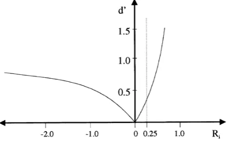
The ratios of potential to kinetic energy storage as a func-tion ofRi, as deduced by Hocking (1992), are shown graph-ically in Fig. 5.
We therefore recognize that even when theRidependence ofγ is understood, there is not general agreement about the details of the relationship. Different authors have produced different relationships, and we cannot resolve these differ-ences here. Our preference is to use Eq. (32).
If Richardson number measurements are not available, then a value of
γ =0.4 (33)
is recommended as a reasonable compromise, since it cor-responds approximately with a Richardson number of 0.25 according to (32). We therefore see that we are once again
Fig. 5. The ratio of the potential energy and kinetic energy spectral densities,
d, plotted as a function of the Richardson number,Ri. Note that the
ratio tends to infinity asRiapproaches 1, and tends to 1 asRiapproaches
negative infinity (from Hocking, 1992).
returning to an assumption of a constant value forγ, but this approach is adopted simply because it is often not possible to measureRiwith sufficient resolution. It is fairest to think of this as a mean value forγ. It is often the best we can do, but is definitely an inferior approach to proper use of Ri in determiningγ.
6.2 An alternative way to determine εεεεεεεε using spectral
fitting around the spectral knee
Because of uncertainties in regard to application of the pre-viously discussed “Cn2”method, L¨ubkenet al.(1993), and Lubken (1997) developed an alternative method for determi-¨ nation ofε. This method still employs direct measurements of scalar spectra, but in a different manner to that described in the previous section. It has been well-known for many years that if one can measureη, the Kolmogoroff microscale, then one can determineεthrough the relation (7). The kinematic viscosityνis usually taken from empirical atmospheric mod-els. The major difficulty is determination ofηaccurately, be-causeεis proportional toηto the fourth power. For example, an error inηof a factor of 2 means an error inεof a factor of 16. Traditionallyηhas been determined by finding the inner scale,0, and then determiningηthrough (8) using an assumed value forc4. (e.g. Watkinset al., 1988). The value ofc4depends on whether one is measuring velocity fluctu-ations, ionfluctuations, neutralfluctuations or whatever, as seen earlier.
This method fell from favour, however, because there was too much uncertainty in determining0. Different extrapola-tion schemes produced different values. Lubken has recently¨ attempted to solve this difficulty byfitting a carefully pre-scribed function to the Fourier-spectrum of the time series of neutral densityfluctuations measured by a moving rocket (expressed as a function of the spectral angular frequencyω) viz.
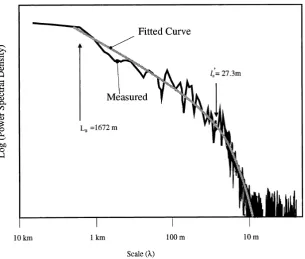
An angular frequency ofωcorresponds to a spatial scale in the turbulence along the track of the rocket with “wave-length”equal to 2πvr/ω. Here,(5/3) = 0.90167; vr is the rocket speed; fα = 2.0, andk0 = 2π/0, where0 is a length scale closely related to0. The denominator in the last multiplicative term was introduced as an attempt to al-low the inertial range to run smoothly into the viscous range, and is somewhat ad-hoc. Because this is so, it is necessary to exercise some care in the meaning of0. L¨ubkenet al.
Fig. 6. Experimental andfitted spectra for rocket measurements of neutral densityfluctuations. The smooth curve shows afit assuming a Heisenberg model in the viscous range. Buoyancy and inner scales are also shown (adapted from Lubken, 1997).¨
wherek0 =2π/0, and the termχLaccounts for the fact that the spectral“knee”need not occur directly at a wavenumber ofk0.
By fitting this functional form to the measured spectra, L¨ubkenet al. (1993), and L¨ubken (1997) were able to de-termine0 to fairly high accuracy. The value of0can be determined independently ofCn2and fα. They then assumed that0 is proportional to0, and so used a variation on (8) viz.
0=c4η. (36)
They used c4 = 9.90 to get η, and thence determined
ε. This choice required some knowledge about the Prandtl number, and there is some uncertainty in this regard. L¨ubken
et al.(1993) and L¨ubken (1997) used 0.82, whilst Hill and Clifford (1978) suggest 0.72. The latter result is the correct choice if it is recognized that the temperature spectra and the neutral density spectra are identical in form. An example of the measured andfitted spectra is shown in Fig. 6.
However, it is appropriate at this juncture that we make some comments about the functionW(ω). This function is designed to describe both the inertial range of the spectrum as well as the viscous range, plus the transition between them. It is proportional toω−7at largeω, which limits its usefulness to
some degree. For example, if one requires the variance of the third derivative of the spatialfluctuations, (as is sometimes sought in turbulence studies), then it involves an integral over allωofW multiplied byω6, which is an integral ofω−1, and is therefore infinite. Higher order derivatives have similar infinities. Indeed, Heisenberg’s original proposal for aω−7
form at high wavenumbers was criticized by, for example, Batchelor, for reasons like this. Furthermore, Heisenberg’s formula was really only supposed to apply to energy spectra,
whereas L¨ubkenet al.have adapted it to scalar spectra. The possibility of such infinite integrals places some limits on the usefulness of this particular function; if this functional form is indeed used, it is necessary that the user places some sort of artifical limit on the integrals, or assumes that the spectrum changes form yet again at some point well into the viscous range.
Indeed, the optimal choice of W(ω) requires additional discussion, and should at this stage be considered indeter-minate. L¨ubken found by experimentallyfitting the data to different functions that the so-called“Heisenberg” theoret-ical form described by Eqs. (34) and (35) gave the bestfit, although his original papers also discussed a model due to Tatarskii (1971) for the viscous range. However, we have noted doubts about the suitability of the Heisenberg form. Another possibility which well deserves examination is the temperature spectrum of Hill and Clifford (1978). It should be recognized that within turbulence in the free air, the fluc-tuations in temperature and thefluctuations in density should have the same form, since neutralfluctuations due to pressure perturbations are negligible, so this is an excellent candidate. Nevertheless, for now we recognize that L¨ubken’s prefer-ence is to use Eq. (34). We recognize that the chief new contribution from Lubken¨ et al.(1993) and L¨ubken (1997) to measurements of turbulence was to develop a formalism whereby 0 could be determined usingallof the available spectrum, thereby (hopefully) producing higher accuracy.
W. K. HOCKING: DYNAMICAL PARAMETERS OF TURBULENCE 535
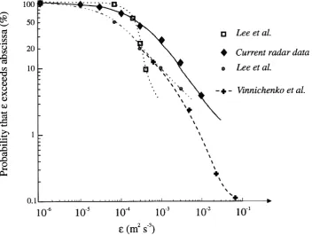
Fig. 7. Cumulative graph ofεin the troposphere (from Hocking and Mu, 1997), using radar data and the theory embodied in Eqs. (10) and (33), as well as various in-situ measurements. Data are compared to Leeet al.(1988) and Vinnichenkoet al.(1973).
the Prandtl number have also been noted above. Addition-ally, becauseεvaries as the fourth power of0, even small errors in estimating0 can lead to considerable errors inε. However, even despite these problems, the method remains one of the more commonly used for rocket studies of tur-bulence. It is only possible to guess at the effects of these systematic errors, although we would hope that the method gives accuracies which are correct to within a factor of 2.
6.3 Application of the newC2
n
C2
n
C2
n
C2
n
C2
n
C2
n
C2
n
Cn2formula to some in-situ data
In this section, we wish to intercompare the two ap-proaches described in Subsections 6.1 and 6.2, since they have been two of the main approaches to determinations of
εby rocket techniques. Previous comparisons have not al-ways shown good agreement, but in each case we have noted recent developments and adjustments, so it will be of interest to see how the two different techniques now compare after these new developments are considered.
The formulae presented in Subsection 6.1, which involve the more proper use ofγ, have been tested in at least a couple of cases, and seem to produce somewhat better estimates than do those which do not properly consider the Richardson-number dependence of this quantity. We shall illustrate some of these, but it should nevertheless be borne in mind that even the tests shown here are not really definitive, and more tests are unquestionably needed. In particular, in these tests we have had to assume thatγ =0.4, whereas it would be much nicer to use actual measured values of the Richardson number made at scales of a few tens to hundreds of metres.
Thefirst such test is shown in Fig. 7, which summarizes results from Hocking and Mu (1997), using tropospheric data. This shows a cumulative distribution of energy
dissipa-tion rates measured by various techniques, including radar. Whilst the data were taken at different sites, and on different occasions, the overall agreement is quite reasonable. Val-ues obtained by radar and shown here, for example, show broadly better agreement that do those which do not use this more recent theory.
A more interesting comparison comes about by examining the same data using two different analysis techniques. We have chosen the rocket data obtained by Thraneet al.(1985, 1987), Lubken¨ et al.(1987), and Blixet al.(1990), which have been nicely tabulated in those references. We have con-verted the energy dissipation rates produced by these authors back to effective structure constants (analagous toC2
Fig. 8. Energy dissipation rates from Thraneet al.(1985), Lubken¨ et al.(1987) and Blixet al.(1990), produced after rescaling according to Eqs. (10) and (33). Rescaled raw data are shown by the symbols“T”. Thefilled squares show median values ofεdue to the original authors, whilst the solid circles show median values using the newer theory. The left and right borders of thefilled area shows 16% and 84% percentiles using the newer theory. The solid lines show estimates for summer and winter due to Lubken (1997), using his procedure for¨ fitting spectra to the data.
the methods described in Subsection 6.2 than do the earlier methods.
7.
The Relation between Diffusion and Energy
Dissipation Rates
The issue of the relation between the rates of diffusion and the rate of energy dissipation in the atmosphere is another area which is often oversimplified. It is often assumed that (11) applies, and that measurements ofεimmediately enable determination of the rate of vertical diffusion, K. Authors vary in their assumed values ofc2, but most (with the possible exception of McIntryre, 1989) generally agree that the value lies between 0.2 and 1.25 (e.g. Fukaoet al., 1994; Lillyet al., 1974; Weinstock, 1981). We will not dwell too much on the actual value ofc2here; it is premature to specify it more precisely than has been done here, although a value of 0.8 is commonly used.
A more important matter here is not whatc2is, but rather
whether (11) applies at all. The methods by which diffu-sion can take place are far more complex than simple three-dimensional turbulent diffusion. The reasons for this lie in
two main facts;first, turbulence is very intermittent both tem-porally and spatially, and very often occurs in thin layers in the middle atmosphere. These thin layers are often separated by regions which are either only weakly turbulent or even laminar. Secondly, the processes which induce diffusion can themselves be scale dependent.
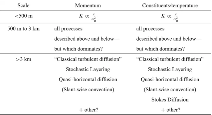
These factors mean that there are several ways in which diffusion can occur. Table 1 summarizes some of these pro-cesses, and we will now elaborate briefly upon them.
Thefirst important factor is the spatial and temporal in-termittency. This effect has been demonstrated in Hocking (1991, 1996b), after adaptation from Desaubies and Smith (1982). These authors show how an ensemble of gravity waves can act together to produce regions of instability sep-arated in height by regions of stability, with layer thicknesses of a few tens of metres out to a kilometre or so. Examples of experimental studies of such layering are also discussed there-in.
W. K. HOCKING: DYNAMICAL PARAMETERS OF TURBULENCE 537
Table 1. This table shows some of the various processes which are normally grouped together as“diffusive”processes in the atmosphere. Classical turbulent diffusion is only one such process, and at large scales is not necessarily even one of the most important. At intermediate scales (500 m to 3 km), all of these processes occur, but we have left question marks here to indicate that it is uncertain just which of all these processes dominates in this regime.
Scale Momentum Constituents/temperature
<500 m K∝ ε ω2 B
K ∝ ε ω2
B
500 m to 3 km all processes all processes
described above and below— described above and below—
but which dominates? but which dominates?
>3 km “Classical turbulent diffusion” “Classical turbulent diffusion” Stochastic Layering Stochastic Layering
Quasi-horizontal diffusion Quasi-horizontal diffusion
(Slant-wise convection) (Slant-wise convection)
Stokes Diffusion
+other? +other?
due to Dewan (1981) and Woodman and Rastogi (1984) sug-gested that the random occurrence of layers produces a Monte Carlo type of intermittent diffusion. In this model, diffusion is not a continuous process, but a step-wise one. First one layer of turbulence forms around a particle of interest, purely due to chance. Turbulent transport of this particle then takes place, possibly to the edge of the layer, or until the layer dies out. At this time the particle remains fairly stationary, since molecular diffusion is assumed to be very small. Then at a later time, another turbulent layer forms around the particle, and further transport over the depth of that layer is now pos-sible. This process repeats itself over and over. Thus the factors which control the large-scale diffusion are not sim-ply the rates of diffusion across individual layers, but the frequency of occurrence and depth of individual layers (this process is illustrated diagramatically in Fig. 2 of Hocking, 1991). Any determinations of effective diffusion coefficients must take this into account. Proper modelling of the effects of this intermittency remains an important area of research.
Other consequences of the intermittency of turbulence in-clude the possibility that the average rates of diffusivity of momentum and heat may be different, and that the Prandtl number may exceed 1, and perhaps be in the range of 1 to 3 (Fritts and Dunkerton, 1985). This is to say that if one pa-rameterizes the rate of heat transport asKT(∂θ/∂z), where
∂θ/∂zis the mean potential temperature gradient, ignoring the effects of the wave, then the effective coefficient which must be used to describe the rate of diffusion is less than it would be if we properly included the effect of the wave in
∂θ/∂z. This is not so for momentum diffusion, because‘u’ and‘w’are not in phase quadrature. Fritts and Dunkerton (1985) have proposed this process as a way to explain the conclusions of Strobelet al.(1987), in which these authors claim that the turbulent Prandtl number is somewhat in excess of unity in the atmosphere.
Another important means of vertical diffusion is quasi-horizontal diffusion along tilted isopleths. It is well known that horizontal diffusion at large scales is a much faster
pro-cess than vertical diffusion. If the mean gradients are tilted, then this horizontal diffusion attains a vertical component, and can lead to an effective vertical mixing. Admittedly a particle which starts at an altitude of z km, and finally achieves a height ofz+ζ km, may also have drifted hori-zontally a distance equal to perhaps hundreds of timesζ, but nevertheless this still produces an effective vertical mixing.
Another important process which can produce significant diffusion is so-called “Stokes Diffusion”, as proposed by Walterscheid and Hocking (1991) and Hocking and Walterscheid (1993). These authors have shown that even a linear combination of Boussinesq waves produces a dif-fusive-like effect on particles over periods of many hours, and whilst this process is not as strong as classical turbu-lence in causing diffusion at scales of a few tens to hundreds of metres, it becomes a major diffusive effect when applied at scales of many hours. This is because it is not affected by the intermittency of turbulence, and acts just as strongly in laminar regions as it does in turbulent ones. This pro-cess is especially important for diffusion of constituents. If the waves are damped, the diffusive effect becomes even stronger, especially if the damping induces particles to cross between contours of constant potential tempearture; in this case, Stokes diffusion may also be important for momen-tum diffusion. As noted, Table 1 summarizes some of these processes.
8.
Conclusion
Some of the constants traditionally used in turbulence the-ory, and indeed some classical interpretations, have been re-examined. The basis for these formulae have been dis-cussed, showing how some of these constants arise. Appro-priate formulae for application of radar and in-situ measure-ments of turbulence have been presented, including recom-mendations for the most appropriate constants where possi-ble. Where necessary, oversimplifications in current thinking about turbulence have also been pointed out. Without ques-tion, though, all current measurements of energy dissipation rates in the middle atmosphere have uncertainties of some type; a major goal in the next few years should be to de-velop instrumentation which can directly measure velocity fluctuations in-situ down to scales within the viscous range. Only then will it be possible to unambiguously interpret the spectra, and determine turbulent energy dissipation rates with precision.
Acknowledgments. The careful comments and suggestions of two anonymous reviewers were of great help in thefinal preparation of this document. This work was supported in part by the Natural Sciences and Engineering Research Council of Canada.
Appendix A. Velocity Structure Functions
The following appendices summarizes the main struc-ture functions and spectra used in turbulence theory, without proof or derivation.
The first type of function which we will discuss that is commonly used to describe turbulent phenomena is the so-called Structure Function. There are several of these, but the main ones areDandD⊥, which are defined in the following way;
D(r)= |u(x+r)−u(x)|2 (A.1)
and
D⊥(r)= |u⊥(x+r)−u⊥(x)|2, (A.2)
where we imagine traversing the turbulent medium in a straight line and taking point measurements along the way. “Parallel”components refer to measurements of the veloc-ity components with directions parallel to the direction of traverse, and“perpendicular”components refer to velocity components perpendicular to this direction. Isotropy has been assumed in this definition, which is why we considerD
to depend only on the magnituderof the vectorr.
Occasionally a 3-D form of the structure function is some-times used, viz.
Dtot(r)= |u(x+r)−u(x)|2, (A.3)
where the vector difference between displaced components is used. Because there are two perpendicular components, and one parallel component, we may write
Dtot=D+2D⊥. (A.4)
For inertial range, homogeneous,Kolmogoroff-style tur-bulence, we have the following relations.
D =Cv2r2/3 (A.5)
whereC2
v =Cε2/3, andC is close to 2.0 (e.g. Caugheyet al., 1978; Kaimal, 1976). In addition,
D⊥= 4
3C
2
vr2/3, (A.6)
Dtot=
11 3 C
2
vr2/3. (A.7)
There are also a variety of spectral forms which are used as tools in turbulence studies.
Appendix B. Spectral Forms for Velocity
Measure-ments
A variety of spectra are used for turbulence studies. These all have different purposes, and are summarized below for Kolmogoroff-type inertial-range turbulence.
Thefirst important expression is
F(k)=Aε2/3k−11/3 (B.1)
wherek = |k| is the length of the vectork, (and so takes
values between 0 and infinity), and A = 11(83)sin(π3)
24π2 C
0.061C, (Tatarskii, 1971). This is a full three-dimensional function describing the total kinetic energy per unit cell size (due to all three velocity components) in a cell of sized3kat
the end of a vectorkoriginating from the origin. For homo-geneous isotropic turbulence this function is isotropic. Pic-torially one can visualize this as a solid sphere in(kx,ky,kz) -space which has highest density at the centre, and decreasing density as|k|increases, where the density representsF.
Because this function is isotropic, it is often integrated over a shell of radiuskto give a new expression which is
E(k)=4πk2F=αε2/3k−5/3 (B.2)
where α = 4πA = 11(
8 3)sin(π3)
6π C = 0.76655C (e.g. see
Tatarskii, 1971; Batchelor, 1953). Note that we will largely follow Batchelor’s symbol-usage in this document: For ex-ample, we use E(k)dk to represent the total energy in a shell ink-space of thicknessdk, as does Batchelor, whereas Tatarskii (1961, 1971) uses the symbol E to represent the function which we have calledF.
If we useC=2.0, then we have
E(k)=1.53ε2/3k−5/3. (B.3)
Different authors use different values for the constant 1.53—anything between 1.35 and 1.53 are common. Note, however, that if one adjusts this constant then the constant
Calso needs adjustment. I prefer to useC=2.0 because it has at least been measured with good accuracy in the lower atmosphere (e.g. Caugheyet al., 1978)
These equations are fairly simple to understand. However, there are more complex variants. An important adjunct (and in fact a more fundamental expression) is the equation
i j(k)=
E(k)
4πk4 ·(k 2δ
i j −kikj) (B.4)
W. K. HOCKING: DYNAMICAL PARAMETERS OF TURBULENCE 539
or j =2”mean theydirection and“i or j =3”mean the
zdirection. The valuesk1,k2andk3may take both positive
and negative values. Note thatkis the length of the vector from the origin to the point(k1,k2,k3)ink-space, and so
For each of these spectra there is a related covariance func-tion; for example,
where Ri is the aoutovariance function corresponding to
iand wherej = √
−1 in this expression. We will not dis-cuss these various covariance functions in much detail here; the reader is referred to to Tatarskii (1961, 1971), Batchelor (1953) or Lumley and Panofsky (1964) for more elaborate discussions.
For cases of isotropic turbulence, we can integrate i j around a shell of radiuskto give (e.g. Batchelor, 1953, p. 35)
i j(k)=
i j(k)k2d k. (B.6)
For homogeneous, isotropic turbulence, we therefore have
i j(k)=4πk2i j(k). (B.7)
E(k)relates to thei j(and hence to thei j) via the rela-tion
E(k)=1
2(11(k)+22(k)+33(k)). (B.8)
Notice the factor 12; this is introduced so that the integral over all k (i.e. from k = 0 to k = ∞) gives the kinetic energy per unit mass, 12v2
tot. E(k)is unique in this regard—
other spectra have normalizations which do not involve this factor of12. For example,
∞
0
11(k)dk=u21 (B.9)
whereu1refers to the velocity component in thexdirection.
Sometimes (B.8) is also written as
E(k)= 1 and33(e.g. Lumley and Panofsky, 1964, p. 28).
The above spectra are useful from a conceptual viewpoint, but are often hard to determine experimentally, since they require a full three-dimensional description of the turbulent field in all three velocity components. That is, they require knowledge of all three velocity components at all points in space. This is often difficult (if not impossible) to measure.
Therefore, we also look for spectral analogues to the structure functions which were described earlier for a one-dimensional pass through the turbulentfield.
To begin, if we have a detector which moves in a straight line through a patch of turbulence, and it records the velocity components parallel to the direction of motion (in analogy to the process described in connection with Eqs. (A.1) to (A.3)),
and then we Fourier transform the resultant spatial series, we obtain (for Kolmogoroff turbulence) the function
11(k1,0,0)=α11ε2/3|k1|−5/3 (B.11) where α11 = 559α = 0.1244C. This is in fact a one-dimensional function which we will denote asφp, viz.
φp(k1)=α11ε 2/3|k1|−5/3. (B.12)
It is important to note that this is not the same as
11(k1,0,0). Whilst both refer to spectral densities along thexaxis,11(k1,0,0)refers to spectral densities dueonly
to“waves”with the phase-fronts aligned perpendicular to the
xaxis. On the other hand, 11(k1,0,0)(andφp(k1)) refer to the spectral density at wavenumberk1due to contributions
of“waves”ofallorientations which cross thexaxis. These concepts are fundamentally different. In fact,
i j(k1,0,0)=
i j(k1,k2,k3)dk2dk3. (B.13)
Likewise, if we find the spectrum for the velocity com-ponents perpendicular to the direction of motion during this traverse, we produce
φt(k1)= 22(k1,0,0)=α22ε 2/3|k1|−5/3 (B.14) whereα22 =43α11.
Additionally, for the choice ofC =2.0 described above, we have
φp(k1)= 11(k1,0,0)=0.25ε2/3|k1|−5/3
−∞<k1 <∞, (B.15)
φt(k1)= 22(k1,0,0)=0.33ε2/3|k1|−5/3
−∞<k1<∞. (B.16) In the case of isotropic turbulence, there is no preferred axis, so that these formulae are not restricted to any particular axis.
Because of the obvious symmetry, many experimentalists often“fold”their spectral densities at negative wavenumbers over onto their positive ones, and so do not differentiate be-tween positive and negative signs for the wavenumber. Then we obtain the following functions:
φ wherekαare absolute values of wavenumbers along the di-rection of travel of the probe.
Note that Eqs. (B.11), (B.12), (B.14), and (B.15) to (B.18), have“k−5/3”laws, but so does (B.2). However, these equa-tions are conceptually different; (B.2) represents an integra-tion over a shell of radiusk in three-dimensionalk-space, whilst (B.15) to (B.18) represent spectra determined by a probe moving in a straight line through the turbulence. Nev-ertheless, it is a common mistake for novice researchers to confuse the two spectra, when they speak of the“k−5/3”law,