R E S E A R C H
Open Access
A parameter estimation algorithm for LFM/
BPSK hybrid modulated signal intercepted
by Nyquist folding receiver
Zhaoyang Qiu
*, Pei Wang, Jun Zhu and Bin Tang
Abstract
Nyquist folding receiver (NYFR) is a novel ultra-wideband receiver architecture which can realize wideband receiving with a small amount of equipment. Linear frequency modulated/binary phase shift keying (LFM/BPSK) hybrid modulated signal is a novel kind of low probability interception signal with wide bandwidth. The NYFR is an effective architecture to intercept the LFM/BPSK signal and the LFM/BPSK signal intercepted by the NYFR will add the local oscillator modulation. A parameter estimation algorithm for the NYFR output signal is proposed. According to the NYFR prior information, the chirp singular value ratio spectrum is proposed to estimate the chirp rate. Then, based on the output self-characteristic, matching component function is designed to estimate Nyquist zone (NZ) index. Finally, matching code and subspace method are employed to estimate the phase change points and code length. Compared with the existing methods, the proposed algorithm has a better performance. It also has no need to construct a multi-channel structure, which means the computational complexity for the NZ index estimation is small. The simulation results demonstrate the efficacy of the proposed algorithm.
Keywords: Nyquist folding receiver, LFM/BPSK hybrid modulated signal, Parameter estimation, Signal characteristics
Abbreviations: ADC, Analog to digital converter; BPSK, Binary phase shift keying; CSVR, Chirp singular value
decomposition ratio; FA, Frequency agile; LFM, Linear frequency modulation; LOS, Local oscillator; LPI, Low probability interception; MCRLB, Modified Cramer Rao lower bound; NRMSE, Normalized root mean square error; NYFR, Nyquist folding receiver; NZ, Nyquist zone; RF, Radio frequency; SFM, Sinusoidal frequency modulation; SNYFR, Synchronous NYFR; SVD, Singular value decomposition; ZAM, Zhao, Atlas, and Marks; ZCR, Zero crossing rising
1 Introduction
Currently, the electromagnetic environment is becoming increasingly complex and many modern radar signals have very high carrier frequencies or wide operating bandwidths [1, 2]. In order to intercept the modern radar signals, some receiver architectures have been proposed in the past few decades [3, 4]. The wideband non-cooperative receivers should have the capability of wideband receiving. A typical wideband receiver is the channelization structure, which adopts a set of analog band-pass filters to reduce the bandwidth of each chan-nel and samples each chanchan-nel with a low-speed analog to digital converter (ADC) using filter bank [4].
However, this kind of structure needs a huge amount of equipment. For the purpose of realizing wideband moni-toring with a small amount of equipment, the Nyquist folding receiver (NYFR) architecture is proposed and it can realize wideband monitoring using one ADC [5, 6]. The NYFR modulates the received analog signal in the front-end of the receiver, maps the Nyquist zone (NZ) information to the modulation bandwidth of the signal, and then samples the modulated signal.
Based on the NYFR structure, the output signal pro-cessing using wavelet transform has been studied [7]. Then, some new NYFR architectures using different local oscillator (LOS) modulation types have been pro-posed. Synchronous NYFR (SNYFR) structure using simplified LOS has been proposed and its output can be processed more easily because of the synchronous LOS
* Correspondence:[email protected]
School of Electronic Engineering, University of Electronic Science and Technology of China, Chengdu, China
[8]. Other LOS modulation types such as binary phase shift keying (BPSK) LOS and noise sequences are pro-posed [9, 10], which can improve the performance of NYFR because the bandwidths of these LOS modula-tions remain unchanged.
The NYFR can realize wideband receiving with a small amount of equipment, but the information of LOS modulation will be added on its output [8], and its out-put will be more complex compared with the conven-tional receiver. Some convenconven-tional radar signals such as linear frequency modulation (LFM) signal and frequency agile (FA) signal intercepted by the NYFR have been in-vestigated, and the parameter estimation methods using multi-channel structure have been proposed [8, 11].
Meanwhile, many low probability interception (LPI) radar waveforms have been designed. Linear frequency modulated/binary phase shift keying (LFM/BPSK) hybrid modulated signal is a novel kind of LPI radar signal. It has a double spread spectrum and has been applied in some radar and fuse systems [2]. For the parameter estimation of LFM/BPSK signal intercepted by the conventional receiver, an algorithm based on Zhao, Atlas, and Marks (ZAM) transformation has been studied [12]. However, for the parameter estimation of LFM/BPSK signal intercepted by the NYFR, there has been no public report.
Therefore, considering the increasing complexity of radar waveform and the growing demand of wideband receiving, it is necessary to study the parameter estima-tion of LFM/BPSK signal intercepted by the NYFR. The LFM/BPSK signal intercepted by the NYFR is a typical non-stationary signal. For a non-stationary signal, a common processing idea is the time-frequency analysis. However, many time-frequency methods can achieve op-timal results only for the particular modulation types [13]. Because the LFM/BPSK signal intercepted by the NYFR contains the LOS modulation, it may be difficult to find a time-frequency kernel which is optimal for the NYFR output directly. In this paper, we will study this problem in another way and make full use of the NYFR prior information which is neglected in [8] and [11]. We will model the LFM/BPSK signal intercepted by the NYFR based on the signal self-characteristic and the
NYFR prior information, and propose a parameter esti-mation algorithm which has different estiesti-mation steps compared with the existing NYFR output parameter estimation algorithm [8, 11].
This paper is organized as follows: Section 2 inves-tigates the NYFR architecture and the LFM/BPSK hybrid modulated signal intercepted by the NYFR. Section 3 gives the parameter estimation methods for each modulations of the NYFR output. Section 4 is the algorithm steps for the parameter estimation of the NYFR output. Section 5 gives the simulation results and the corresponding analyses, and we con-clude in Section 6.
2 NYFR architecture and NYFR output signal analysis
2.1 NYFR architecture
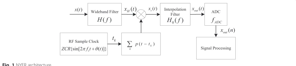
The NYFR architecture [5] is shown in Fig. 1.
In Fig. 1, The NYFR uses zero crossing rising (ZCR) voltage time to control the radio frequency (RF) sample
clock and generate the RF LOS p(t) which is a
non-uniform sampling LOS with a certain modulation type. As long as the modulation information of the LOS remains unchanged, we can simplify the LOS as [8]
p tð Þ ¼ X∞
k¼−∞
δðm tð Þ−2πkÞ ð1Þ
where m(t) = 2πfst+θLOS(t) +φLOS, k is an integer, fs is the LOS carrier frequency which equals the value of NZ bandwidth when the input signal is complex, define (−fs/ 2,fs/2) as the 0th NZ, hence, (kfs−fs/2,kfs+fs/2) is the kth NZ,θLOS(t) is the LOS modulation, andφLOS is the LOS initial phase.
Firstly, the input analog signal x(t) is filtered by a pre-select filterH(f). Then,x(t) is mixed by the non-uniform LOS and we havexs(t) =xH(t)p(t), wherexH(t) is the
out-put of the pre-select filter. The non-uniform sampled sig-nalxs(t) is filtered by an interpolation filterH0(f) with pass band (−fs/2,fs/2) and we obtainxout(t) which contains the LOS modulation information as the output of the NYFR [5]. Finally,xout(t) is sampled by the ADC whose sampling rate isfADCto get the discrete NYFR output.
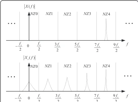
The input signal can be recovered by xout(t) and the NZ information [6]. Figure 2 illustrates the spectrum of
the input signal x(t) and the spectrum of the
non-uniform signalxs(t) which contains the NZ information.
The NYFR output is equal to the spectrum of xs(t) in
the 0th NZ afterXs(f) is filtered byH0(f). 2.2 LFM/BPSK signal intercepted by the NYFR
Let us denote the LFM/BPSK hybrid modulated signal as the NYFR input and it can be expressed as [2]
x tð Þ ¼Aej2πfctþjπμ0t2þjϕð Þþt jφ0 ð2Þ
where t∈[0,T), T is the signal duration, fc is the sig-nal carrier frequency, μ0 is the chirp rate, ϕ(t) is the BPSK modulation and its value is 0 or π, and φ0 is the initial phase.
According to [5], sinusoidal frequency modulation (SFM) is selected as the NYFR LOS modulation, which means m(t) = 2πfst+mfsin(2πfsint) +φLOS in (1),
where mf is the modulation coefficient, fsin is the
modulation frequency, and φLOS is the LOS initial
phase. Considering the LFM/BPSK signal in (2), the output signal of the interpolation filter H0(f) in Fig. 1 can be expressed as [8]
xoutð Þt
¼Aej2πðfc−kNZfsÞtþjπμ0t2þjϕð Þt−jkNZmfsin 2πð fsintÞ þjφ0−jkNZφLOSþw tð Þ
ð3Þ
where kNZ is the NZ index which can indicate the ori-ginal carrier frequency of the input signal [5],t∈[0,T),T is the signal duration, and w(t) is the additive white Gaussian noise [8].
From (3), the NYFR output signal contains three modu-lations (i.e., LFM/BPSK/SFM), and it turns to be more complex compared with the input signal (i.e., LFM/BPSK).
Nevertheless, for the SFM modulation part in (3), the only
unknown parameter is the NZ indexkNZ. For the LFM/
BPSK signal intercepted by a non-cooperative radar signal receiver, the main parameters that need to be estimated are the chirp rate, the carrier frequency, and the code length. Besides, the code length can be calculated by the positions of the phase change points. Thus, the chirp rate, the NZ index, the carrier frequency, and the code length in (3) are the parameters needed to be estimated in this paper. To simplify the following derivation, the initial phase in (3) is omitted.
The ADC sampling rate fADC in Fig. 1 satisfies the
Nyquist sampling theorem and the sampling interval is TADC= 1/fADC, the number of the total sampling points can be computed as N=fADCT. Hence, the discrete ex-pression of (3) is
xoutðnTADCÞ
¼Aej2πðfc−kNZfsÞðnTADCÞþjπμ0ðnTADCÞ2þjϕðnTADCÞ−jkNZmfsin 2ðπfsinðnTADCÞÞ
þw nTð ADCÞ
ð4Þ
wheren= 0,⋯N−1.
3 NYFR output signal parameter estimation
For the NYFR output signal in (4), it contains three modulations (i.e., LFM, BPSK, and SFM). Normally, the time-frequency transform is employed to extract the sig-nal characteristics for a non-stationary sigsig-nal. Because the NYFR output in our paper contains three modula-tions, some time-frequency transform methods cannot achieve an optimal result. For instance, the modulations of BPSK and SFM in the NYFR output signal cannot be extracted properly by using fractional Fourier transform [14] which is suitable for the LFM modulation. Mean-while, ZAM works well for the BPSK modulation [12], but it is poor for the LFM modulation [13]. In addition, the time-frequency representation of (4) is no longer a straight line, which may lead to the polynomial curve fit-ting method [12] failing to estimate the chirp rate. Therefore, it may be difficult to find a time-frequency kernel which is optimal for the three modulations simul-taneously. In this paper, we will focus on the self-characteristic and the prior information of the NYFR output signal to estimate the parameters in (4) instead of the time-frequency transformation method.
3.1 Chirp rate estimation based on CSVR spectrum As to the NYFR output signal parameter estimation steps, the existing algorithm constructs a multi-channel architecture to remove the LOS modulation by estimat-ing the NZ index through extractestimat-ing frequency domain feature for each channel firstly and then estimates other parameters using conventional methods [8, 11]. This Fig. 2Spectra of the NYFR input signal and the non-uniform
algorithm regards the LOS modulation information as a redundant part and neglects the known information in it, which means the periodic characteristic of the LOS modulation. In addition, the accuracy of chirp rate esti-mation using the existing method will be affected by the NZ index estimation result. In order to improve the chirp rate estimation performance, we will estimate the chirp rate directly by using the LOS periodic informa-tion instead of estimating the NZ index firstly.
The square processing is applied to the data in (4) to elim-inate the BPSK modulation, which meansejϕðnTADCÞ2¼1. The carrier frequency in (4) can be written asf0=fc−kNZfs and we have
xsqðnTADCÞ
¼A2ej2π2f0ðnTADCÞþjπ2μ0ðnTADCÞ2−j2kNZmfsin 2πð fsinðnTADCÞÞ
þw′nT ADC
ð Þ
ð5Þ
where w′(nTADC) = 2xout(nTADC)w(nTADC) +w2(nTADC) is the noise after the square processing. To simplify the following discussion, the noise part is omitted.
Because the SFM modulation partmfsin(2πfsint) in (5) is known, the LOS modulation period can be calculated as 1/ fsinand the number of points in one LOS modulation period isNc=fADC/fsin. In addition, for the NYFR structure,fsinand fADCare the prior parameters, thus we can set Nc=fADC/ fsin∈Z+, andMc= floor(N/Nc), where floor(⋅) means choos-ing the integer part of N/Nc, Mc∈Z+, and Mc<Nc. The
above setting implies the number of signal points we use in this section isMcNc, and if the input data lengthN>McNc,
we selectMcNcpoints and omit the remaining points.
Ac-cording to the LOS periodic characteristic, we can model the data in (5) as anMc×Ncmatrix
Xc¼
xsqð Þ0 ⋯ xsqðNc−1Þ
xsqð ÞNc ⋯ xsqð2Nc−1Þ
⋮ ⋱ ⋮
xsqððMc−1ÞNcÞ⋯ xsqðMcNc−1Þ 2
6 6 4
3 7 7
5 ð6Þ
The relationship between the elements in the pth row and theqth row inXccan be calculated as
In addition, becauseNc=fADC/fsin, (7) can be written as xsqðpNcþnÞ
xsqðqNcþnÞ ¼e
j2π2f0ðpNc−qNcÞTADCþjπ2μ0½ðpNcþnÞ2T2ADC
−ðqNcþnÞ2T2ADC þj2kNZmf½sin 2ðπfsinnTADCþ2πqÞ
−sin 2ðπfsinnTADCþ2πpÞ
¼ej2π2f0ðpNc−qNcÞTADC þjπ2μ0½ðpNcþnÞ2T2ADC −ðqNcþnÞ2T2ADC
ð8Þ
From (8), it can be observed when (8) has no LFM modulation part, the quotient of the elements in thepth
row and the qth row will be a constant. Therefore, we
can construct a matrix
SLFMð Þ ¼μ
sLFMð Þ0 ⋯sLFMðNc−1Þ
sLFMð ÞNc ⋯sLFMð2Nc−1Þ
⋮ ⋱ ⋮
sLFMððMc−1ÞNcÞ⋯ sLFMðMcNc−1Þ
2 6 6 4
3 7 7 5
ð9Þ
wheresLFMð Þ ¼n e−jπ2μðnTADCÞ 2
,μis an argument. Then, we have
Yð Þ ¼μ SLFMð Þ μ Xc ð10Þ
where * is the Hadamard product. When μ=μ0, Y(μ0) = SLFM(μ0) Xcwill become an SFM signal matrix and we callSLFM(μ0) as the matching matrix.
Once the constructed matrix SLFM(μ) meets the
matching matrix, (10) will be a matrix whose row ele-ments are equal to the data in one LOS modulation period. Then the singular value decomposition (SVD) of (10) can be computed as Yð Þ ¼μ UYΣYVHY [15], where ΣY is an Mc×Nc diagonal matrix and we call it as the
singular values matrix, the singular values are λ1;λ2;⋯;
λMc and λ1≥λ2≥⋯≥λMc. Based on the SVD ratio (SVR) spectrum [15, 16] and the LOS periodic characteristic, we define the chirp SVR (CSVR) spectrum as
Pð Þ ¼μ λ21
λres
ð11Þ
whereλres¼λ 2 2þ⋯þλ2Mc
Mc−1 .
Considering the noise-free situation, when μ=μ0, the first singular value λ1 in ΣY will achieve its maximum and the rest singular values are 0. We call λ1 is the principle singular value and other singular values are the non-principle singular values. While μ≠μ0, the periodic
xsqðpNcþnÞ xsqðqNcþnÞ ¼
A2ej2π2f0ððpNcþnÞTADCÞþjπ2μ0ððpNcþnÞTADCÞ2−j2kNZmfsin 2ðπfsinððpNcþnÞTADCÞÞ
A2ej2π2f0ððqNcþnÞTADCÞþjπ2μ0ððqNcþnÞTADCÞ2−j2kNZmfsin 2ðπfsinððqNcþnÞTADCÞÞ
¼ej2π2f0ðpNc−qNcÞTADCþjπ2μ
0ðpNcþnÞ 2T2
ADC−ðqNcþnÞ 2T2
ADC
þj2kNZmffsin 2½πfsinððqNcþnÞTADCÞ−sin 2½πfsinððpNcþnÞTADCÞg
characteristic of the LOS in each row ofY(μ) will be dis-turbed by the LFM modulation, and consequently, the non-principle singular values ofY(μ) will be non-zero ac-cording to the energy conservation theory [16]. Therefore, we can search the peak of CSVR spectrum in (11) whose argument is the chirp rate and the estimated chirp rate is
^
μ0¼ arg
μ fmax P½ ð Þμ g
One issue to note is that when μ is close to μ0, Y(μ) will approximate an SFM signal. In order to keep the non-periodic characteristic of LFM signal in Y(μ) when
μ≠μ0, we need to guarantee that the bandwidth of LFM signal in Y(μ) is wide enough. Because the chirp rate is unknown, the longer of the signal length we use will bring the wider of the LFM signal bandwidth, which means we can get a better resolution capability for the CSVR spectrum if we use more signal data. Because we can ob-tainμ0by scanning different values ofμand the interval value ofμis not limited by the data length in (5), we say the CSVR spectrum has the property of super resolution.
Considering the situation that the data in (5) contain noise, the singular values of Y(μ) will be affected by it. When μ=μ0, the non-principle singular values of Y(μ) will be non-zero, and whenμ≠μ0, the non-principle sin-gular values will also be affected by noise. Therefore, the purpose that we useλres in (11) rather thanλ22 in [16] is
to reduce the noise effect to the non-principle singular values through average operation.
Let us analyze the complexity of CSVR spectrum. Let Nsearchbe the number of the chirp rate scanning points. For each scanning point, the flop count [17] for Hadamard product isMcNc. Because the CSVR spectrum only requires
the singular values of Y(μ) and the singular vector matrix
UYandVYneed not be computed, the flop count for
com-putingΣYis 2McN2cþ2N3c[17]. The flop count for average operation isMcand the computational complexity of peak
search isNsearch. Thus, for the proposed method, the total number of flops is Nsearch2McN2cþ2Nc3þMcNcþMc and the computational complexity of peak search isNsearch. In addition, some fast SVD methods [18, 19] may enhance the computational speed.
Then, let us compare the computational complexity of chirp rate estimation using an existing method [8]. Firstly, the existing method requires constructingL channels and the flop count for constructing the channel needsNL mul-tiplications. Then, for each channel, it needs fast Fourier transform whose flop number isN2 log2ð ÞN , instantaneous auto-correlation whose flop number isN, and peak search whose computational complexity isN. The computational complexity of maximum peak finding for theLchannels is Land the SFM demodulation for the input signal requires N multiplications. Finally, the computational complexity
of chirp rate estimation step requires N2 log2ð Þ þN N flops and Nsearch. Thus, for the existing method, the total number of flops isL N þN2 log2ð ÞN þNþN2 log2
N
ð Þ þN and the computational complexity of peak search isLN+L+N.
Although the computational complexity of proposed method is larger than the existing method, the estimation accuracy of the proposed method will be better than the existing method because of the super resolution property. In addition, because the chirp rate is estimated directly in the proposed method, its estimation performance will not be affected by the NZ index estimation result. In contrast, the existing chirp rate estimation method using multi-channel structure needs NZ index estimation result and its performance will be affected by it.
3.2 NZ index estimation based on matching component function
Once the chirp rate has been obtained, the NYFR output hybrid modulated signal can be simplified via the de-chirp method. In order to estimate the carrier frequency, we need to get the NZ index first. The de-chirp signal is assumed as sdechirpðnTADCÞ ¼e−jπ2μ^0ðnTADCÞ
2
, n= {0, 1,⋯,McNc−1}
and we use the data in (5) with the same length to operate the de-chirp process. Omit the noise part and we have
xdeðnTADCÞ
¼xsqðnTADCÞsdechirpðnTADCÞ
¼A2ej2π2f0ðnTADCÞþjπ2ðμ0−μ^0ÞðnTADCÞ2−j2kNZmfsin 2πð fsinðnTADCÞÞ
Because the CSVR spectrum has super resolution capability, the transfer error of chirp rate is small and xde(nTADC) can be written as
xdeðnTADCÞ ¼A2ej2π2f0ðnTADCÞ−j2kNZmfsin 2ðπfsinðnTADCÞÞ
xde(nTADC) is an SFM signal and the unknown parame-ters are the NZ indexkNZ and carrier frequency f0. For the NZ index estimation, the multi-channel structure is a common method [8,11]. This method requires Fourier transform and peak search in frequency domain for each channel. It regards the SFM modulation part as a redun-dancy and neglects the self-characteristic of SFM signal. Here, we will use the self-characteristic of SFM signal and propose an NZ index estimation method using matching component.
According to the LOS prior information, construct a signal
sSFMðnTADC;kÞ ¼ej2kmfsin 2ðπfsinðnTADCÞÞ ð12Þ
ydeðnTADC;kÞ ¼sSFMðnTADC;kÞxdeðnTADCÞ
¼A2ej2π2f0ðnTADCÞþj2ðk−kNZÞmfsin 2ðπfsinðnTADCÞÞ
To simplify the following derivation, denote n=nTADC and the instantaneous auto-correlation ofyde(nTADC,k) is
R nð ;kÞ ¼ydeðn;kÞydeðnþτ;kÞ ¼A4e−j2π2f0τej2ðk−kNZÞmf½sin 2ðπfsinnÞ
−cos 2ðπfsinnÞsin 2ð πfsinτÞ−sin 2ðπfsinnÞcos 2ðπfsinτÞ ð13Þ
Define the matching component function as
PNZð Þ ¼k
According to the self-characteristic of SFM signal, we
have ejksin 2ðπf0nÞ¼
X∞
m¼−∞
Jmð Þk ejm2πf0n, where J
m(⋅) is the
Bessel function withmorder. Based on (13), (14) can be expressed as
when k≠kNZ, because the modulation coefficient can be set as |mf|≥1, we have Jm1 ðk−kNZÞmfð1−cos 2ð πfsinτÞÞ
ponent function PNZ(k) will achieve its maximum and
we call the constructed signal sSFM(nTADC,kNZ) as the matching component. The peak of PNZ(k) indicates the NZ index estimation result.
It should be noted that in order to avoid Jm(⋅)≡0 in
(16), we should make sure 1−cos(2πfsinτ)≠0 and sin(2πfsinτ)≠0 in (16). Therefore, we need to guarantee 2πfsinTADCτ≠2πz,z∈Z, which meansτ≠zfADC/fsin. Ap-parently, we should also avoid τ→zfADC/fsin to prevent 1−cos(2πfsinτ)→0 and sin(2πfsinτ)→0, where→means going close to. This is the selection criterion for the value of shift lengthτ. Because the LOS modulation fre-quencyfsinand the sampling frequency fADCare known, the shift length τ can be set as τ≠zfADC/fsin and it should be far away from zfADC/fsin, z∈Z to satisfy the above requirements.
Furthermore, let us consider the modulation coefficient mf in (16). As we analyzed before, when k≠kNZ, we
is very small, according to the characteristic of Bessel func-tion, we have Jm1 ðk−kNZÞmfð1−cos 2ð πfsinτÞÞ
guaranteed. Therefore, in order to guarantee that the matching component function has a good performance, we should make sure that |mf| is not too small. This is the
rea-son we set |mf|≥1 above.
^
kNZ¼ arg
k fmax PNZ½ ð Þk g
The flop count of the proposed method for
instantan-eous auto-correlation and summation are McNc and
McNc−τ, respectively. In addition, the NZ index
estima-tion needs to search L points to find the peak. Hence, for the proposed method, the total number of flops is 2McNc+McNc−τ and the computational complexity of
peak search isL.
As to the method in [8], from the analysis in Section 3.1, the total number of flops is L N þN2 log2ð ÞN and the computational complexity of peak search is LN+L. Be-cause McNc≤N and L≪N, the proposed method has a
smaller computational complexity.
According to the LOS information and the estimated
NZ index k^NZ, the LOS modulation in (11) can be
demodulated and (11) will become a single carrier signal. Using Fourier transform to estimate the carrier fre-quency and we can obtain the result 2^f0. Hence, the car-rier frequency of the input LFM/BPSK signal can be calculated as^fc¼f^0þ^kNZfs.
3.3 Phase change point estimation based on matching code and subspace
For the BPSK modulation, we not only need to estimate the code length, but also want to obtain the position of each phase change point. This section will present a phase change point estimation method for the BPSK modulation with high accuracy using matching code and subspace orthogonal property.
The chirp rate μ^0 and the NZ index ^kNZ have been
already estimated. Let us reconsider the data in (4) and construct a signal is the noise part. Because the NZ index estimation result is an integer, we can assume k^NZ¼kNZ and it has no transfer error. Since the carrier frequency ^fc of the NYFR input signal has been obtained, the estimation of the carrier frequency in (19) can be computed as ^
f0¼^fc−^kNZfs.
Generally, we can denote xB(n) =xB(nTADC). We re-definen= 1,⋯Nand omit the initial phase. The data in
(19) can be separated into several segments and the length of each segment is Ns which is shorter than the
points of one code length. The method in [20] can be employed to obtain the coarse estimation of the code length and determine the segment length Ns. However,
this method can only give the code length estimation and it has no capability to give the position of each phase change point. The number of the data segments
can be calculated as Num = floor(N/Ns). We redefine
p= 0, 1,…, Num−1 and the signal data in the (p+ 1)th segment can be written as
xNsð Þ ¼ ½xn BðnþpNsþ1Þ;xBðnþpNsþ2Þ;…;
whereDB is the BPSK modulation matrix. If there is no phase change point in the BPSK modulation matrix,DB will become a unit matrix. In this paper, we mark the unit matrix asI.
A BPSK modulation matrix Dð Þ ¼ks diag
ejθ1;ejθ2;…;ejθi;…;ejθNs
can be constructed, where i
= 1,…,Ns and θi¼ π0 ii≥<kks s
, 1≤ks≤Ns, which
im-plies that the phase change point in D(ks) will be
pre-sented point by point ati=ks with the moving ofks. To
estimate the phase change point in one segment, two situations should be taken into consideration:
Under this circumstance, the position of the phase change point in DB is assumed as kphase, 1 <kphase
<Ns. Whenks=kphaseinD(ks),D(kphase)DB= ±Iand we callD(ks) is the matching code ofDB. Meanwhile,
whenks≠kphase, we haveD(kphase)DB≠±I.
(2)The data in one segment have no phase change point, which meansDBhas no phase change point.
Under this condition, when ks= 1 or ks=Ns, we have
D(ks)DB= ±I, which implies D(ks) will match DB when
ksis at the edge of the data segment. Whenks=kphase= 1 orks=kphase=Ns, we also mark D(ks) as the matching codeD(kphase).
Therefore, combining (20) andD(kphase) yield
Dkphase
where w″ is the noise part. The above equation can be rewritten as
where the chirp rate transfer error matrix is
DΔμ0¼diag½ejπΔμ0ðnþpNsþ1Þ
2
;ejπΔμ0ðnþpNsþ2Þ2 ;…; ejπΔμ0ðnþpNsþNsÞ2
and the driving vector is
Að Þ ¼ f0 1;ej2πf0;…;ej2πf0ðNs−1Þ
h iT
Because the carrier frequency^f0 has been already esti-mated, we can construct a signal s^f0ð Þ ¼n e
subspace ofRsscan be computed and it can be denoted
asG.
Firstly, let us consider (21) is noise free. According to the noise subspaceGfroms^f0ð Þn, we get
The result of (23) will be affected by the chirp rate transfer error Δμ0 and the carrier frequency transfer error f0−^f0. If Δμ0= 0 and f0¼^f0, we have DHΔμ0 ¼I
Then, we can define the phase search pseudo-spectrum as achieve its maximum and the corresponding peak pos-ition^kscan be calculated by
^
become the matching code and the corresponding point ^
ksis the estimated position of the phase change point in one data segment. If the data in one segment have no phase change point, Phase(ks) will show a peak at the
first or the last point of the data segment from the ana-lysis of situation (2).
According to (24) and (25), if the transfer errors of chirp rate and carrier frequency are 0, the width of the peak in (25) will be one point. Thus, the phase search pseudo-spectrum can obtain an accurate estimation re-sult and its peak width is independent of the data seg-ment length comparing with the wavelet transform method whose peak width is decided by the length of the scale [19].
However, if the chirp rate transfer error Δμ0 is not 0, the transfer error matrix of chirp rate will be no longer a unit matrix. With the increasing ofΔμ0, DΔμ0 will be far away from a unit matrix. Meanwhile, (24) will also be far away from 0and the width of the peak in (25) will be expanded. In addition, if the carrier frequency transfer error is not 0, the orthogonal relation between
AH(f
carrier frequency will deteriorate the accuracy of phase change point estimation.
Fortunately, because the CSVR spectrum is a super resolution method, the chirp rate transfer errorΔμ0→0. In addition, because the NZ index estimation result is an integer and it has no transfer error, we have ^f0→f0. Hence, (24) can be written as
D kphase
xNsð Þn
HG→0 ð
27Þ
Then, let us consider the signal xNwð Þn containing noise. According to (23) and (27), if D(ks) matches DB,
we get
D kphase
xNsð Þn
HG→0þw″HG
IfD(ks) does not matchDB, we have
Dð Þks xNsð Þn
½ HG→xH
Nsð ÞnDHð Þks Gþw″HG
Thus, under the condition of noised signal, the phase search pseudo-spectrum in (25) can still achieve its peak whenD(ks) matchesDB.
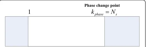
After the peak search process is completed in one data segment, there is one issue to be considered. The pos-ition of the phase change pointkphase may locate at the first or the last point of the data segment. This situation is shown in Fig. 3.
For this condition, the following process can handle this issue.
For the (p+ 1)th data segment, when the phase search pseudo-spectrum shows a peak at k^s¼pNsþ1 or ^ks ¼pNsþNs, we can assume c is a small integer, c> 1, and reselect the data from pNs+ 1 +c to pNs+Ns+c.
The reselected data can be written as
~
xNsð Þ ¼n
xBðnþpNsþ1þcÞ;xBðnþpNsþ2þcÞ;…;
xBðnþpNsþNsþcÞT
ð28Þ
The result of (26) can be recalculated using the data from (28). The peak position of the phase search pseudo-spectrum using the data in (28) is denoted as ^
ksð Þag and we have
^
ksð Þag ¼ arg
ks
max 1
Dð Þks ~xNsð Þn
½ HGGHD k
s
ð Þ~xNsð Þn
½
( )
ð29Þ
This process is illustrated in Fig. 4.
If the reselected data segment shows a peak at the first point (i.e., k^sð Þag ¼1), let ^ksð Þag ¼Ns, which means if the data in (28) have no phase change point, the position of the peak is always at the end of this segment.
If the distance between k^sð Þag and the last point of the reselected data segment is not equal toc, we regard that the last point of the (p+ 1)th data segment is not the phase change point. Otherwise, the last point of the (p+ 1)th data segment covers the phase change point. For the first point of the next data segment, if the distance between ^ksð Þag and the last point of the reselected data segment is not equal to c−1, we regard that the first
point of the (p+ 2)th data segment is not the phase
change point. Otherwise, the first point of the (p+ 2)th data segment covers the phase change point.
Finally, let us compare the computational complexity of our method with the method using the Haar wavelet transform [21]. We focus on the data in one segment. The number of the points in one segment is still as-sumed as Ns. Besides, we also assume that the wavelet
scale contains Ns points. Because the noise subspace in
(25) is fixed, we consider the computational complexity of matrix multiplication in one data segment. Thus, the computational complexity of the proposed method needsNs[Ns+ 4Ns(Ns−1) + 2(Ns−1)] number of flops in
one data segment. For the method in [21], the computa-tional complexity needs 2N2
s number of flops for one
wavelet scale. Although the proposed method requires a larger computational complexity, its estimation result can achieve a higher accuracy. Since the phase change point in one data segment has been estimated, the next section will give the code length estimation process.
4 Algorithm steps
For the LFM/BPSK hybrid modulated signal intercepted by the NYFR in (4), the proposed parameter estimation algorithm steps are as follows:
1) For the NYFR output signal in (4), the square method is employed and the signal data whose length isMcNcpoints are selected as shown in (5).
Model the data in (5) as the matrixXcwhich is shown in (6) based on the periodic characteristic of the LOS modulation and construct the LFM matching matrixSLFM(μ) expressed in (9). Estimate the chirp rate^μ0by computing the CSVR spectrum based on (11);
2) The de-chirp process using^μ0can be operated to eliminate the LFM modulation of the signal in (5). Construct the matching component as shown in (12). Based on the matching component function PNZ(k) in (14), the NZ index estimation result^kNZ can be obtained. According to the LOS information
and^kNZ, the NYFR output carrier frequency^f0and
the input hybrid modulated signal carrier frequency fccan be estimated;
3) Construct the signal in (22) using^f0and calculate its noise subspaceG. Demodulate the signal in (4) using the estimated^μ0and^kNZ. The data in (20) can be obtained by dividing the demodulated signal into Num segments and setp= 0.
4) For the data frompNs+ 1 topNs+Nsin the (p+ 1)th
data segment, calculate the phase search pseudo-spectrum in (25) usingGand the constructedD(ks).
Find the peak position ^ks;p in the (p+ 1)th data segment. Ifk^s;p∈ðpNsþ1;pNsþNsÞ,k^s;p∈Zþ, record
^
ks;p. If^ks;p¼pNsþ1 or^ks;p¼pNsþNs, reselect
the data frompNs+ 1 +ctopNs+Ns+cand find the
corresponding peak positionk^ð Þs;agp according to the
reselected data and (29). Decide whether the edge of the (p+ 1)th data segment covers the phase change point and record k^ð Þsag;p . If the edge covers
the phase change point, record ^ks;p¼pNsþNs or ^
ks;pþ1¼ðpþ1ÞNsþ1; otherwise, set ^ks;p as a null value. Then, p=p+ 1. If p< Num−1, continue this step and process the next data segment; 5) Finish the phase change point estimation of the
Num data segments and obtain^ks;p andk^ð Þs;agp ,p= 0,
…, Num−1, where^ks;p is the phase change point
estimation in the (p+ 1)th data segment andk^ð Þsag;p
is the recorded position of the phase change point estimation result using the reselected data of the (p+ 1)th segment. In order to make full use of the estimation results, usek^s;pand^ksð Þag;p ,p= 1,…, Num
−1, to modify the false phase change points which are caused by the noise. For the recorded^kð Þs;agp , if ^
ks;pþ1∈ðpNsþ1;pNsþ1þcÞandNs−cþ^ks;pþ1≠
^
kð Þsag;p ,^ks;pþ1 is regarded as a false position and mark it as a null value. Finally, we obtain all the phase change points in the LFM/BPSK signal;
6) Omit the estimation result of the first data segment and the number of the rest estimated phase change
points is Num−1. Find the nearest two^ks;p which are not null and mark them as^ks;p1 andk^s;p2, where
p2>p1. Thus the code length of the hybrid modulated
signal isLB¼ðp2−p1ÞNsþ^ks;p2−k^s;p1.
5 Simulation results
In this section, numerical simulations are conducted to demonstrate the merits of the proposed scheme. SFM signal is adopted as the LOS modulation for the NYFR, and the LOS modulation can be expressed asm(t) = 2πfst
+mfsin(2πfsint) +φLOS, where the LOS carrier frequencyfs is 1 GHz, the LOS modulation coefficientmfis 4, the LOS
modulation frequency fsin is 10 MHz, the LOS initial
phaseφLOSis 0, and the number of the monitored Nyquist zones is 10.
The hybrid modulated LFM/BPSK signal is s tð Þ ¼A
ej2πfctþjπμ0t2þjϕð Þþt jφ0 , where the carrier frequency fc is
4.1 GHz, the chirp rate μ0 is 50 MHz/μs, the BPSK
modulation ϕ(t) is [-1 -1 1-1 -1 1 1-1 1 1], the signal amplitude Ais 1, the signal initial phase φ0is 0, the sig-nal length is 1 μs, and the ADC sampling rate fADC is 2 GHz.
5.1 Chirp rate estimation simulation
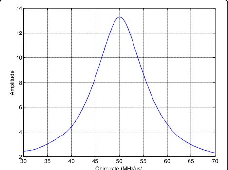
The CSVR spectrum of the NYFR output signal based on Section 3.1 is given. Here, we set the signal-to-noise ratio (SNR) as 7 dB and the scanning chirp rate reso-lution is 0.01 MHz/μs. Considering the LOS parameters, we have Nc=fADC/fsin= 200 and Mc=N/Nc= 10. Hence, the signal can be modeled as a 200 × 10 matrix and the CSVR spectrum is shown in Fig. 5.
From Fig. 5, when the scanning chirp rate is equal to
50 MHz/μs, the CSVR spectrum meets its maximum,
which agrees the analysis of (10). In addition, when the scanning chirp rate is far from the signal chirp rate, the
30 35 40 45 50 55 60 65 70
2 4 6 8 10 12 14
Chirp rate (MHz/µs)
e
d
util
p
m
A
non-periodic LFM component will affect the singular values. Hence, the non-principle singular values will in-crease and λres in (11) will rise up. Moreover, according
to the energy conservation theory, the principle singular
value λ1 will decrease. Thus, the amplitude of CSVR
spectrum will drop with the increasing distance between the scanning chirp rate and the signal chirp rate.
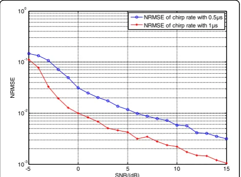
Figure 6 illustrates the normalized root mean square error (NRMSE) of chirp rate estimation using CSVR spectrum with different signal lengths. The signal lengths are 1 and 0.5μs, respectively, and other parame-ters remain unchanged. The number of Monte Carlo experiments is 200.
In Fig. 6, the NRMSE of chirp rate estimation using 1-μs signal length is less than 10−2 when the SNR is greater than 0 dB, which shows a better performance
compared with the signal whose length is 0.5 μs. The
reason is the bandwidth of LFM component with
1-μs length is wider and its resolution capability is bet-ter. This simulation result proves the discussion in Section 3.1.
5.2 NZ index estimation simulation
The NZ index estimation result based on the matching component function in Section 3.2 is given in Fig. 7. The SNR is still set as 7 dB. Because the number of Nyquist zones has been set as 10, the argument inPNZ(k) can be set as k= 0, 1,⋯, 9. According to the known fsin= 10MHz andfADC= 2GHz, the shift lengthτcan be set as 100 points in (13).
Considering the simulation parameters, the real NZ
index should be kNZ= round(4.1GHz/1GHz) = 4. From
Fig. 7, it is shown when k= 4, PNZ(k) achieves its
maximum. Apparently, the proposed method can obtain the correct NZ index.
Let us focus on the amplitude value of the peak in Fig. 7. Because the selected signal length in our simula-tion is McNc= 2000, the shift length is τ= 100 and the
signal amplitude isA= 1, the theoretical value ofPNZ(k) can be computed as PNZ(kNZ) =A4(NcMc−τ) = 1900
when k=kNZ= 4 from (17). Meanwhile, the peak value of the simulation result in Fig. 7 is 1914 and we have 1914≈PNZ(kNZ). Hence, this simulation proves the correctness of (17). In addition, comparing frequency domain peak search for each channel in [8], the pro-posed method only needs one-dimensional search for the matching component function and the computa-tional complexity of our method is small. Once the chirp rate and the NZ index are estimated, we can estimate the carrier frequency according to Section 3.2.
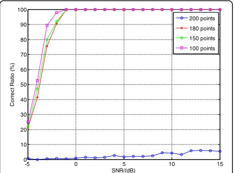
Besides, in order to examine the shift length selection criterion in Section 3.2, we set different shift length values to show how the shift length affects the correct ratio of NZ index. The values of shift lengthτare set as 100, 150, 180, and 200 points, respectively. Other pa-rameters remain unchanged. Figure 8 gives the correct ratio of NZ index using a different shift length.
From Fig. 8, the estimation correct ratio of NZ index has the best performance when the shift length τ= 100, which implies the distance betweenτandfADC/fsin= 200 is the largest. When the distance betweenτandfADC/fsin is smaller, the correct ratio of NZ index will decrease. Particularly, when τ=fADC/fsin= 200, the Bessel function in (16) will become Jm(⋅)≡0 and the matching
compo-nent function will lose its capability. This simulation proves our discussion about the shift length selection criterion in Section 3.2.
Furthermore, to show the effect of modulation coef-ficient mf to the matching component function,
differ-ent modulation coefficidiffer-ents are used to estimate the
NZ index. The values of modulation coefficient mf
-5 0 5 10 15
10-3 10-2 10-1 100
SNR/(dB)
E
S
M
R
N
NRMSE of chirp rate with 0.5µs NRMSE of chirp rate with 1µs
Fig. 6NRMSE of chirp rate estimation with different signal lengths
0 1 2 3 4 5 6 7 8 9
0 200 400 600 800 1000 1200 1400 1600 1800 2000
X: 4 Y: 1914
NZ number
e
d
util
p
m
A
are set as 0.1, 0.5, 1, 4, and 10, respectively. Other parameters remain unchanged. Figure 9 presents the correct ratio of NZ index using different modulation coefficient.
From Fig. 9, the correct ratio of NZ index with mf=
0.1 is less than 90 % when the SNR <3 dB. Meanwhile, the results with other modulation coefficients have bet-ter performances and their correct ratios are greabet-ter than 90 % when the SNR >−3 dB. The reason of this phenomenon is that the value of the Bessel function in (16) will approach to 1 when |mf|→0 and the
relation-ship in (18) cannot be guaranteed. When |mf| > 0, the
re-lationship in (18) can be guaranteed, which implies the NZ index estimation performances (exceptmf= 0.1) are
better and tend to be the same. This simulation proves the discussion about the modulation coefficient selection criterion in Section 3.2.
5.3 Phase change point and code length estimation simulation
Figures 10 and 11 illustrate the normalized phase search pseudo-spectra with phase change point and without phase change point in one segment. The SNR is still 7 dB and the segment length in Section 3.3 is Ns= 80.
Figure 10 represents the eighth segment and Fig. 11 is the ninth segment. According to the simulation parame-ters, the code length of BPSK is 200 points.
From Fig. 10, whenk^s¼40, the phase search pseudo-spectrum Phase(ks) reaches its maximum and this peak
corresponds to the phase change point of the third and the fourth codes in [-1 -1 1-1 -1 1 1-1 1 1], which means the position of the phase change point is (p−1) ×Ns+
ks= (8−1) × 80 + 40 = 600. From Fig. 11, Phase(ks) shows
a peak at the first point when the data segment has no phase change point. The data in the ninth segment corres-pond to the signal points from 640 to 720, and obviously, there is no phase change point in such data segment. After we present the phase search pseudo-spectrum in one segment, Fig. 12 gives the estimated phase change point position ^ks;p of the NYFR output signal in each data segment. The number of the data segments in Fig. 12 is Num−1 = floor(2000/80)−1 = 24.
The horizontal axis in Fig. 12 indicates the data segment number and the vertical axis represents the position of each phase change point. When the value of vertical axis is 0, it means there is no phase change point in that seg-ment. In Fig. 12, five phase change points have been esti-mated and the position of each phase change point can be calculated based on the segment length and the vertical axis values. In addition, from the 5th and 20th segments, we can see the edges of these data segments cover the phase change points. However, our method can still esti-mate these covered phase change points.
-5 0 5 10 15
Fig. 9Correct ratio of NZ index using different modulation coefficients
Fig. 10Data segment contains one phase change point
-5 0 5 10 15
5.4 Parameter estimation performance
At last, let us consider the performance of the proposed method. Although there is no public report for the par-ameter estimation algorithm of the LFM/BPSK signal intercepted by the NYFR, we still can employ the algo-rithm using multi-channel structure in [8] and the method in [21] as the comparisons. The shift lengthτis 100 points and the LOS modulation coefficient mf is 4.
The correct ratio of NZ index, the NRMSEs of chirp rate, and carrier frequency and the correct ratio of code length are given, respectively. The SNR is set from−5 to 15 dB, and 500 Monte Carlo trials are used for each SNR value.
Figure 13 compares the NZ index correct ratio of the proposed method with that of the method in [8]. The proposed method performs better than the method in [8] when SNR <0 dB, because the method in [8] esti-mates the NZ index using the amplitude value in fre-quency domain which is sensitive to the noise.
Figure 14 illustrates the NRMSEs of chirp rate and carrier frequency estimation results using the proposed method, the method in [8], and the modified Cramer Rao lower bound (MCRLB) [22], respectively. As indicated in the result, when SNR >−2 dB, the chirp rate estimation of our method can achieve NRMSE <0.01. However, the chirp rate estimation method in [8] yields large estimation errors when SNR <0 dB due to the NZ index estimation transfer error. In detail, when SNR <0 dB in Fig. 13, the correct ratio of NZ index of [8] is smaller than 90 % and the NZ index transfer error will lead to a poor chirp rate estimation performance, which can be seen from Fig. 14. In contrast, the proposed method estimates chirp rate dir-ectly and its performance will not be affected by the NZ estimation result. In addition, because the CSVR spectrum is a super resolution method, the proposed method is closer to the MCRLB.
Figure 14 also reveals that the proposed method per-forms better than the method in [8] in estimating the carrier frequency when 2 dB > SNR >−2 dB, because the proposed method has a better NZ index estimation performance. When the SNR is greater than 2 dB, the performances of both methods are almost the same due to the same carrier frequency estimation process (i.e., Fourier transform).
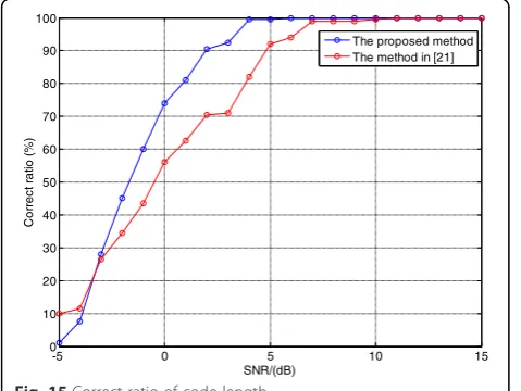
Figure 15 presents the correct ratio of code length es-timation using the proposed method and the method in [21]. Here, the correct ratio of code length means when the code length estimation result strictly equals (1 × 10− 6
/10) ×fADC= 200 points, we regard that the estimation result is correct. From Fig. 15, the proposed method out-performs the method in [21] and the correct ratio of the proposed method is greater than 90 % when SNR >2 dB, because the peak width of phase search pseudo-spectrum is narrower.
In summary, for the LFM/BPSK hybrid modulated sig-nal intercepted by the NYFR, the proposed method can
0 5 10 15 20 25
Fig. 12Phase change point in each data segment
-5 0 5 10 15
Fig. 13Correct ratio of NZ index
0 10 20 30 40 50 60 70 80
obtain accurate estimation performances for the chirp rate, the carrier frequency, the NZ index, the code length, and the phase change points when SNR is greater than 2 dB.
6 Conclusions
On the basis of the NYFR prior information and signal self-characteristic, the parameter estimation algorithm of LFM/BPSK hybrid modulated signal intercepted by the NYFR has been proposed. We make full use of the LOS prior information to model the NYFR output signal and propose the CSVR spectrum to estimate the chirp rate directly. Then, according to the self-characteristic of the SFM modulation, the matching component function has been designed to estimate the NZ index and the carrier frequency. Finally, the matching code and subspace or-thogonal property have been employed to obtain the position of each phase change point and the code length. Furthermore, we also analyze the parameter selection criteria and the computational complexity for each step.
Comparing the existing NYFR output signal parameter estimation algorithm, the proposed algorithm avoids constructing multi-channel architecture and estimating the NZ index firstly. Meanwhile, the proposed scheme can achieve a higher accuracy compared with the exist-ing parameter estimation methods. The simulation re-sults show the proposed scheme demonstrates a good performance and prove our analyses. Besides, the esti-mation methods in Sections 3.1 and 3.2 can be used to estimate the parameters of LFM signal intercepted by the NYFR in one NZ as well.
Acknowledgements
The authors thank the National Natural Science Foundation of China for their supports for the research work. The authors also thank the reviewers for their suggestions and corrections to the original manuscript.
Funding
This study was supported by the National Natural Science Foundation of China (61172116 and 61571088) and 863 Project (2015AA7031093B and 2015AA8098088B).
Authors’contributions
ZQ is the first author and corresponding author of this paper. His main contributions include (1) the basic idea, (2) the derivation of equations, (3) computer simulations, and (4) writing of this paper. PW is the second author whose main contribution includes analyzing the derivation of equations and refining the whole paper. JZ is the third author and his main contribution includes analyzing the basic idea, checking simulations, and refining the whole paper. BT is the fourth author and his main contribution includes refining the whole paper. All authors read and approved the final manuscript.
Competing interests
The authors declare that they have no competing interests.
Received: 29 April 2016 Accepted: 9 August 2016
References
1. A Lazaro, D Girbau, R Villarino, Wavelet-based breast tumor localization technique using a UWB radar. Prog Electromagn Res98, 75–95 (2009) 2. D Lynch,Introduction to RF Stealth(SciTech Publishing Inc, Raleigh, 2004),
pp. 336–343
3. J Zhang, J Wu, W Liu, C Qiao, L Wang, Clock study of high speed interleaving/multiplexing data-acquisition system. J Univ Sci Tech China 36(3), 281–284 (2006)
4. SR Velazquez, TQ Nguyen, SR Broadstone, Design of hybrid filter banks for analog/digital conversion. IEEE Trans Signal Process46(4), 956–967 (1998) 5. GL Fudge, RE Bland, MA Chivers et al.,A Nyquist folding analog-to-information
receiver(42nd Asilomar Conference on Signals, Systems and Computers, Pacific Groue, 2008), pp. 541–545
6. M Ray, L Gerald, L Fudge et al., Analog-to-information and the Nyquist folding receiver. IEEE J Emerging Sel Top Circuits Syst2(3), 564–578 (2012) 7. OO Odejide, CM Akujuobi, A Annamalai et al.,Application of analytic wavelet
transform for signal detection in Nyquist folding analog-to-information receiver
(IEEE International Conference on Communications, Dresden, 2009), pp. 1–5 8. D Zeng, H Cheng, J Zhu et al., Parameter estimation of LFM signal intercepted by synchronous Nyquist folding receiver. Prog Electromagn Res C23, 69–81 (2011)
9. X Zeng, D Zeng, H Cheng, B Tang, Intercept of frequency agile signals with Nyquist folding receiver using binary phase shift keying as the local oscillator. IETE J Res58(1), 44–49 (2012)
10. K Long, D Zeng, B Tang, G Gui, Nyquist folding digital receiver for signal interception. IEICE Electron Expr11(2), 1–6 (2014)
11. D Zeng, X Zeng, B Tang, Nyquist folding receiver for the interception of frequency agile radar signal. Int J Phys Sci7(9), 1454–1460 (2012) 12. X Zeng, B Tang, Y Xiong, Interception algorithm of S-cubed signal model in
stealth radar equipment. Chin J Aeronaut25, 416–422 (2012)
-5 0 5 10 15
Fig. 15Correct ratio of code length
-5 0 5 10 15
NRMSE of chirp rate using the proposed method NRMSE of carrier frequency using the proposed method NRMSE of chirp rate using the method in [8] NRMSE of carrier frequency using the method in [8] MCRLB of chirp rate
MCRLB of carrier frequency
13. T Merlin, J Roshen, B Lethakumary, Comparison of WVD based time-frequency distributions, inInternational Conference on Power, 2012, pp. 1–8
14. HM Ozaktas, O Arikan et al., Digital computation of the fractional Fourier transform. IEEE Trans Signal Process44(9), 2141–2150 (1996)
15. PP Kanjilal, S Palit, G Saha, Fetal ECG extraction from single-channel maternal ECG using singular value decomposition. IEEE Trans Biomed Eng44(1), 51–59 (1997)
16. PP Kanjilal, Adaptive prediction and predictive control. IEE Control Eng Ser 52, 321–322 (2008). 474–478
17. GH Golnb, CF Van Loan,Matrix computations(The Johns Hopkins Univ. Press, Baltimore, 2001), pp. 19–20
18. JR Bunch, CP Nielson, Updating the singular value decomposition. Num Math31, 111–129 (1978)
19. MP Holmes, AG Gray, CL Isbell Jr,QUIC-SVD: Fast SVD using cosine trees. Conference on Neural Information Processing Systems, 2008, pp. 673–680 20. S Tang, Y Yu, Fast algorithm for symbol rate estimation. IEICE Trans Commun
e88(4), 1649–1652 (2005)
21. Z Qiu, J Zhu, P Wang, B Tang,Parameter estimation of phase code and linear frequency modulation combined signal based on fractional autocorrelation and Haar wavelet transform. 17th International Conference on Computational Science and Engineering, 2014, pp. 936–939
22. P Wang, D Du, Z Qiu, B Tang,Modified Cramer-Rao bounds for parameter estimation of hybrid modulated signal combining PRBC and LFM. IEEE 17th International Conference on Computational Science and Engineering, 2014, pp. 1029–1033
Submit your manuscript to a
journal and benefi t from:
7Convenient online submission
7Rigorous peer review
7Immediate publication on acceptance
7Open access: articles freely available online
7High visibility within the fi eld
7Retaining the copyright to your article