Multi linear sparse reconstruction for SAR imaging based on higher order SVD

R E S E A R C H

Open Access

Multi-linear sparse reconstruction for SAR

imaging based on higher-order SVD

Yu-Fei Gao

, Guan Gui

, Xun-Chao Cong

, Yue Yang

, Yan-Bin Zou

and Qun Wan

Abstract

This paper focuses on the spotlight synthetic aperture radar (SAR) imaging for point scattering targets based on tensor modeling. In a real-world scenario, scatterers usually distribute in the block sparse pattern. Such a distribution feature has been scarcely utilized by the previous studies of SAR imaging. Our work takes advantage of this structure property of the target scene, constructing a multi-linear sparse reconstruction algorithm for SAR imaging. The multi-linear block sparsity is introduced into higher-order singular value decomposition (SVD) with a dictionary constructing procedure by this research. The simulation experiments for ideal point targets show the robustness of the proposed algorithm to the noise and sidelobe disturbance which always influence the imaging quality of the conventional methods. The computational resources requirement is further investigated in this paper. As a consequence of the algorithm complexity analysis, the present method possesses the superiority on resource consumption compared with the classic matching pursuit method. The imaging implementations for practical measured data also demonstrate the effectiveness of the algorithm developed in this paper.

Keywords: Spotlight SAR imaging, Kronecker constraint, Compressed sensing, HOSVD, Alternating least squares

1 Introduction

Synthetic aperture radar (SAR) is an important detec-tion system in many fields for decades, such as remote sensing, environmental monitoring, and ground mapping [1–4]. Imaging algorithm is the key point of SAR appli-cation, which extracts the scatter coefficients of targets and reconstructs the image of target scene from the radar echoes [5, 6]. On the azimuth direction, a larger aperture can be synthesized by the coherent processing and rel-ative motions between the antenna and targets. For the range direction, the pulse compression is usually applied to obtain a good range resolution. However, the existing methods encounter several challenges in practical applica-tions. For instance, the overwhelming amount of resource requests for storing and operating in receiver since the high sampling rate; in addition, the conventional imag-ing method, such as polar format algorithm (PFA), suffers from the sensibility to sidelobe disturbance, which leads to it being unsuitable for high-resolution imaging. For

*Correspondence: [email protected]

1_{School of Electronic Engineering, University of Electronic Science and}

Technology of China, No. 2006, Xiyuan Ave., West Hi-Tech Zone, Chengdu 611731, China

Full list of author information is available at the end of the article

solving the problem of high demand on hardware, the compressed sensing (CS) framework has been introduced into SAR imaging [7–11], which can extract necessary information at a lower sampling rate than Nyquist limit [12–14]. Furthermore, the CS-based approach is able to accomplish SAR imaging with the low sidelobe and pos-sess the robustness to noise [15–20]. But the existing methods only utilize the spatial sparsity of the observa-tion without taking advantage of structural features of target scene. In 2016, a sparse reconstruction SAR imag-ing method was proposed by Zhao et al., which employed structured sparsity constraint based on Bayesian learning framework [21]. But this method requires rigid condi-tions to ensure model matching; consequently, the imag-ing quality may be worse if observations cannot perfectly match the model selected.

For practical applications of SAR imaging, the scatterers generally tend to be clustered together as blocks. In this paper, a tensor-decomposition-based algorithm is devel-oped to exploit such block sparsity of targets. Tensor decomposition is a kind of higher-order data processing framework which can make use of the multidimensional and highly structured features in signal [22–24]. Recently, combining tensor modeling with sparse reconstruction

is becoming the focus of attention in signal processing. In 2010, Lim and Comon proposed a sparse reconstruc-tion method based on low-rank tensor decomposireconstruc-tion and analyzed the condition of uniqueness for decomposition [25]. In 2011, Duarte and Eldar introduced the Kronecker structure into dictionary constructing, proposing the Kronecker-CS framework [26]. In 2012, Sidiropoulos and Kyrillidis investigated CS theorem with regard to low-rank tensor signal processing, proposing a two-step sparse reconstruction algorithm [27]. In 2013, Caiafa and Cichocki proposed two types of matching pursuit algo-rithms based on tensor decomposition [28]. However, there has been little work in SAR imaging based on sparse reconstruction combined with tensor decomposition. The higher-order CS approach in hyperspectral imag-ing enlightens our study in signal modelimag-ing [26, 29, 30]. In this paper, an imaging algorithm is developed based on higher-order singular value decomposition (HOSVD) [31, 32] with the Kronecker constraint of reflected waves, which can take advantage of the block sparse feature of target scene to gain more robust high-resolution imag-ing performance. The theoretical analysis and simulation experiments verify that the developed algorithm is supe-rior to the reference methods especially in severe condi-tions, which demonstrates the practical significances.

The following is the organization of the rest in this paper: Section 2 illustrates the signal model for spotlight SAR; Section 3 introduces the tensor modeling based on HOSVD; Section 4 proposes the algorithm by introducing the multi-linear block sparse reconstruction and the pre-processing scheme for dictionary construction; Section 5 demonstrates several numerical simulations to verify the effectiveness of the proposed algorithm; Section 6 con-cludes this paper.

2 Problem formulation

First of all, several notions of this paper are stated as follows.

• The scalar is indicated by italic letter, e.g.,x. • The vector and matrix are indicated by bold italic

letters, e.g.,x,X.

• The tensor is indicated by calligraphic capital letter, e.g.,X.

• The index of a set is indicated by script letter, e.g.,X. • x0is thel0-norm which indicates the number of

nonzero elements inx.

• XFis the Frobenius norm of the tensorX, denoting the square root of the sum of the absolute squares of its elements.

• The operator⊗denotes the Kronecker product between matrices.

• The operator×ndenotes the mode-n product between tensor and matrix, wheremode is considered as the order of tensor data [33].

• For a third-order tensorX ∈CM×N×P_{, defineX} (1)as a rectangular matrix combined allP slices ofXunder mode-1, i.e.,X(1)=[X1,X2, ...,XP]T ∈C(PN)×M; similarly,X(2)andX(3)denote the unfolded matrix of

Xalong mode-2 and mode-3, respectively.

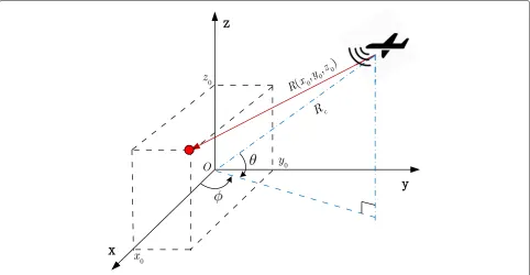
This paper considers spotlight SAR for capturing the structural information of the SAR targets, which is a beamforming-based observation system [34–36]. The radio beam will be pointed to the observation scene con-tinuously while the aircraft carrying SAR flying cross over the target scene. The geometry of such model is shown in Fig. 1.θ andφ indicate the azimuth and pitch angles of radio wave, respectively.R(x0,y0,z0)represents the

dis-tance between the antenna and target at (x0,y0,z0); Rc represents the distance between the antenna and the cen-ter of the scene. Defining the speed of light as c, then the corresponding propagation time can be written as

τc=2Rc/c.

The received signal can be represented as

y(t,θ,φ)= x,y,z

g(x,y,z)s(t−τ (x,y,z))+e(t), (1)

whereg(x,y,z)is the scattering function of the scatterer located at (x,y,z); s(t) is the autocorrelation function of transmitted signal; e(t) is the additive noise. For the simplicity, the noise item is not shown in the following content. After transformation to frequency domain, the phase history of the received signal can be represented as

Yf,θ,φ=C(f) sinφ +zf sinθ) is the phase factor. The constant term C(f)=S(f)exp−j2πfτc

can be ignored in the following discussion, whereS(f)is the Fourier transform ofs(t).

Because the parameters in the phase factor of the sig-nal model (2) are coupled, it is needed to implement an interpolation approach for decoupling [34]. Thus, the coordinate conversion is done from polarization to Carte-sian system [37]. Assume there areM1,M2,M3grid points

in the directions of the axis of x, y, z, respectively, and the numbers of grid points forf,θ,φareP1,P2,P3,

Fig. 1The geometry of spotlight SAR for point scatterers

M=M1×M2×M3,P=P1×P2×P3. Hence, the received

signal model (2) can be written as

y=Ds, (4)

wheres=[g(x1,y1,z1),. . .,g(xM1,yM2,z1),. . .,g(x1,y1,zM3)

,. . .,g(xM1,yM2,zM3)]T. Without loss of generality,

con-sidering the (p1p2p3,m1m2m3)-th element of matrix D

is exp−j4_cπxm1up1+ym2vp2+zm3wp3

, thus D = D3⊗D2⊗D1, by which the Kronecker structure can be

shown explicitly. As a consequence, the received signal can be rewritten as

y=(D3⊗D2⊗D1)s. (5)

3 Tensor decomposition for SAR imaging

In signal processing field, a tensor indicates the multi-linear data with more than two modes. This paper adopts the HOSVD [24, 31], which can be represented as

Y =S×1D1×2D2×3. . .×NDN, (6) whereYdenotes the received signal tensor. For a HOSVD, the operation criterion is

min

S,{Dn}Nn=1

Y−S×1D1×2D2×3. . .×N DN2F. (7)

The one-dimensional expansion of a tensor is stacking all elements along the mode-1, i.e.,y = vecY(1)

. Thus, (6) can be rewritten as

y=(DN ⊗DN−1⊗. . .⊗D1)s. (8)

The equation above indicates that the HOSVD of a ten-sor signal is equivalent to a linear representation with Kronecker dictionary. It is defined that aK-sparse repre-sentation of signaly is existed on a dictionaryD, if the following condition is true:

y=Ds, s.t.s0K, (9)

whereKis named as sparsity. Because the rows of dictio-nary is less than the columns, this is an underdetermined system; hence, no unique solution ofsexists. However, if the signal possesses sparsity, a solution may be obtained under the following condition [38],

K < 1 2

1+ 1

μ (D)

, (10)

where μ (D) = max i=j di,dj

_{, representing the} coher-ence coefficient of dictionaryD; here,di,dj

denotes the inner product of di and dj. When the dictionary pos-sesses Kronecker structure, i.e., D = DN ⊗ DN−1 ⊗

. . .⊗D1, the coherence coefficient should be μ (D) =

max{μ1,μ2,. . .,μN}, withμn=μ (Dn), n=1, 2,. . .,N. It is demonstrated that the total coherence depends merely on the factor matrix with the largest coherence coefficient for a Kronecker dictionary [39, 40].

Kn(n=1,. . .,N) columns in the factor matrices of its HOSVD need to be computed, i.e.,

Y=S×1D1×2D2×3. . .×NDN,

represents a subset of index for mode-n(n=1, 2,. . .,N).

The above definition demonstrates that the nonzero elements of core tensor are included in a subtensor S(I1,I2,. . .,IN). Here,In= ments along each mode of Y are the second and fourth elements along each mode ofX, respectively, i.e.,Ypicks the corresponding elements inX indexed by{In}3n=1. As

a consequence, y isK-sparse with regard to Kronecker dictionary D = (DN⊗DN−1⊗. . .⊗D1), where K =

K1K2. . .KN. It should be noted that the definition ofblock sparsehere is different from the conventional definition of block sparse representation for one-dimensional signal. For the latter, the data is distributed in adjacent data seg-ments [41–43], which is not necessary at the situation of block sparsity based on tensor frame. In 2009, Eldar and Mishali introduced the concept of block sparsity in one-dimensional signal [44]. For an underdetermined system y = Dx, assuming that the coefficient vectorx consists of a series data segments with given length{dm}Mm=1and

denoting m-th segment as x[m], the segment is called block. Define the block sparsel0-norm ofx asx0,b = ferent from this definition of conventional block sparsity, the multi-linear block sparsity considers mainly the addi-tion to the multi-linear structural restraint as interpreted in Definition 1.

It has been demonstrated that the recovery method based on Kronecker dictionary has much less strict requirements for coherence than the classic matching pur-suit method with the same sparsity in regard to signal reconstruction, and it is deduced that the former has the higher successfully recovery bound [28, 45]. In addi-tion, by utilizing the structural information in each mode, the method based on tensor decomposition can perform robustly under the condition of high coherence [46].

4 The proposed algorithm

In higher-order signal processing, taking advantage of sparsity is becoming a research trend due to the curse

of dimensionality problem [24, 47, 48]. Recently, apply-ing CS scheme is risapply-ing in high-resolution radar imag-ing field, which can reconstruct the source signal from the undersampled measurements. The CS-based imaging method must solve an ill-posed linear inverse problem by using the sparsity of targets [12, 49–51]. However, for the large-scale data case, the classicl0 algorithm has to

encounter many computing problems. For instance, con-sidering a scene of 1024×1024 observation points, the classic sparse reconstruction method must process the data up to 1,048,576 length, which is a large-scale linear system demanding numerous computational resources. A more efficient approach is investigated in this paper to ameliorate the above problems. As mentioned previously, the SAR imaging model maintains Kronecker structure and the scatterers in target scene are usually clustered together as blocks. As a result, we can take advantage of the block sparsity feature, building a sparse reconstruction SAR imaging algorithm based on Kronecker dictionary.

After decoupling procedure, the reflected signal can be formulated in the tensor form as explained in (8). Then, the nonzero scatter coefficients need to be recovered from the received signalY, i.e., finding a(K1,K2,. . .,KN) -block sparse representation corresponding to dictionar-ies Dn(n=1, 2,. . .,N). According to the compressed sampling theory, only a few rows need to be randomly extracted from the dictionary.

To begin with, we adopt a preprocessing approach for constructing the dictionaries from observation data. Let E =Y−S×1D1×2D2×3. . .×NDN, then we have

thus, (7) can be rewritten as

max

By utilizing alternating least squares (ALS) algorithm, (12) can be solved in an iterative scheme. Such algorithm fixes(N−1)factor matrices in each iteration and updates the remaining component via least square approach, then repeats this process until the condition of convergence is satisfied. Z(1) and ensuring that the singular values are arranged in descending order, then the first M1 left singular

vec-tors of Z(1) give the estimation ofD1 [52]. Next, fixing

the same way. Repeat this procedure until all dictionaries are obtained.

Then, letBn = Dn(:,In), n = 1, 2,. . .,N, then the received signal model can be rewritten as

ˆ

y=(BN⊗BN−1⊗. . .⊗B1)snz, (14) where snz ∈ RK denotes the vector of nonzero coeffi-cients. As a consequence, the solution of the problem can be presented as

then a sparse representation can be guaranteed if

(K0μ (D))N <2−(1+(K0−1) μ (D))N[28], whereD=

(DN ⊗DN−1⊗. . .⊗D1).

In addition, a more efficient calculation step can be employed. The relationship between Snz and Y can be described as

where Snz is the tensor reshaping form ofsnz. Defining Q = Snz ×1 I ×2 BecauseBT₁B1 is a self-adjoint matrix, there exists a fast

algorithm which can obtain the solution of Qby utiliz-ing Cholesky decomposition [53]. Next, unfold Q to a rectangular matrix along mode-2:

, similar to the above analysis, then we have BT₂B2W(2) = Q(2). The solution of W can be found by

utilizing Cholesky decomposition likewise. In accordance with this scheme, afterNsteps, the estimation ofSnzwill be obtained.

The algorithm flow is shown in Algorithm 1. During iterations, it is necessary to guarantee that the nonzero elements of core tensor are concentrated within a sub-set of index. When the convergence criterion is achieved, all nonzero elements and the corresponding index set can be obtained as the results, and the expected scatter coefficients will be recovered as well.

Algorithm 1Higher-order SVD-based SAR imaging algorithm

Require: observation dataY; the number of grid points {Mn,Pn}Nn=1; the number of maximum nonzero

entrieskmax; the threshold of error.

Ensure: scatter coefficient estimation Sˆ; dictionaries {Dn}Nn=1.

1: Initialize the dictionaries

2: Decouple the observation signal and construct the tensor dataY.

mates of nonzero coefficients snz by utilizing Cholesky decomposition (16), (17);

18: Reshapesnzto the tensor formSnz;

19: Compute the residualE←Y−Snz×1B1×2B2×3

. . .×NBN; 20: k←k+1; 21: end while

22: Reconstruct the scatter coefficientsSˆfrom Snz and index set I = {I1,I2,. . .,IN} , satisfying that

ˆ

S(I1,I2,. . .,IN)=Snz.

The key step of Algorithm 1 is estimating the nonzero coefficients by least squares procedure, which needs no more than2NkkN+P+1+Nk2operations. By contrast, the orthogonal matching pursuit (OMP) algo-rithm [38, 54] needs kNPN+3kN operations in this step. And in the residual update step, it is required to calculate Snz ×1 B1 ×2 B2 ×3 . . . ×N BN and sub-tract it from Y, which needs PN(2k+1) operations for the present algorithm, whereas the requirement for OMP algorithm is PN2kN+1. Consequently, for a multi-linear(K0,K0,. . .,K0)-block sparse reconstruction

of iteration of the present algorithm is NK0. By

con-trast, OMP algorithm requiresK₀Niterations for the same condition. The complexity analysis results indicate that the present algorithm can be used to estimate the scat-ter coefficients with much lower computational resource requirement compared with classic matching pursuit algorithm.

5 Experiments and discussion

This section will provide several numerical experiments to verify the effectiveness and performance of the pro-posed algorithm. The experiments include two parts: (1) SAR imaging realizations for ideal point scatter-ing model and practical measured data and (2) perfor-mance comparisons between the proposed algorithm and the existing algorithms, including PFA [55, 56], OMP [38], and CoSaMP [57]. The PFA method is a kind of classic SAR imaging method which has good real-time response, although susceptible to the sidelobe effect. OMP and CoSaMP are both sparse reconstruction algo-rithms which can achieve the super-resolution perfor-mance, but they need to pay much more computational cost. The hardware configuration for the simulation sys-tem is Intel Core i7-5500U 2.4GHz CPU, 8GB RAM, Windows 10 OS.

5.1 SAR imaging realizations

Two groups of numerical experiments are demonstrated in this section. One tests the SAR imaging for ideal point targets, and the other investigates the effectiveness of real-world conditions. The simulation scenario is configured as follows: the center frequency is 9 GHz; the bandwidth is 1 GHz; the frequency resolution is 0.01 GHz; the angle aperture is 5◦; the angle resolution is 0.05◦; the sampling rate is 50%.

5.1.1 Ideal point targets

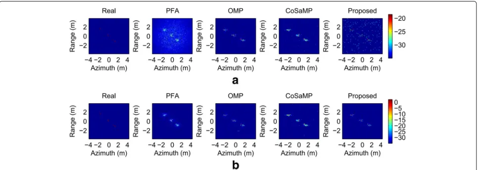
Different SNRs Firstly, the imaging results under dif-ferent SNRs are presented to confirm the feasibility of the proposed algorithm. Twenty ideal point scatterers are deployed in this simulation scenario, located along the diagonal line of the target scene randomly and clustered as three blocks. Corresponding to the settings of the SNR as 3 and 30 dB, the SAR imaging realizations are shown in Fig. 2.

The simulations under different SNRs show the imag-ing qualities of the proposed algorithm and the reference algorithms. When SNR is low, the imaging results of clas-sic matching pursuit algorithms exhibit distinct outliers, and PFA shows severe noisy ambiguity at the same time. As a contrast, the proposed algorithm performs much better under the low SNR condition. When SNR is high, the results of all methods indicate the congruent imaging quality.

Different number of scatterers In this simulation sce-nario, we consider the influence caused by the number of scatterers. The configuration is the same as the previous section, other than fixing the SNR at 10 dB. When the number of scatterers is set to 30 and 150, the SAR imaging realizations are shown in Fig. 3.

It is shown from the simulations that when the num-ber of scatterers is not large, all the methods are able to achieve an acceptable imaging resolution; contrastively, the proposed algorithm can obtain a neater imaging result. However, the scatterers located near the edge of the scene may obscure as the number of scattering points is increasing. The reconstructed scene for the PFA method show more obvious image noise than the matching pur-suit algorithms, and the proposed algorithm can achieve the most accurate images under the same condition.

Fig. 3SAR imaging for ideal point scatterer model under different number of scatterers.a30 scatterers.b150 scatterers

5.1.2 Practical measured data

In this part, a set of experiments based on practical mea-sured data are demonstrated to verify the practicability of the proposed algorithm. The observation target is a crawler-type vehicle. There are three observation angles of a spotlight SAR:

• 77.5◦∼82.5◦, the central angle is80◦ • 87.5◦∼92.5◦, the central angle is90◦ • 97.5◦∼102.5◦, the central angle is100◦

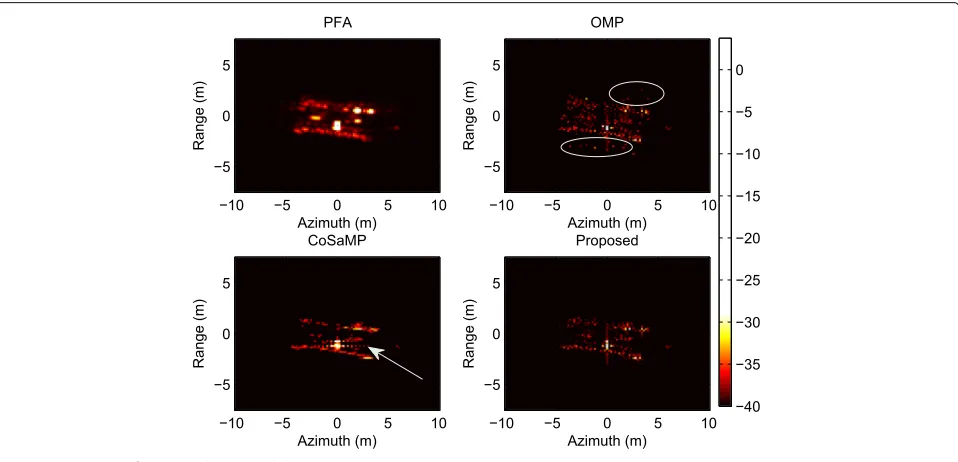
The center frequency and bandwidth are 9 and 1 GHz. As the results, when the central angles are 80◦, 90◦, and 100◦, the SAR imaging realizations are shown in Figs. 4, 5, and 6, respectively.

The imaging results show the availability and superior-ity of the proposed algorithm in real SAR imaging. It is demonstrated that all the sparse reconstruction methods can achieve the higher resolution images than PFA. The latter can merely obtain fuzzy images, especially when the observation angle is not perpendicular to the target scene. Although OMP and CoSaMP are able to achieve the high-resolution results, there exist some problems with these classic matching pursuit techniques. For instance, when the observation angle is 90◦, there is a distinct bright streak that appears on the edge of the target in the imag-ing result of CoSaMP. As indicated by the arrows in Figs. 4 and 6, CoSaMP shows raster lines over the target image at the central region, which will severely influence the recognition of target. In addition, OMP may result in

Fig. 5SAR imaging for practical measured data,_φ=90◦

outliers on the sides of the target, which are marked by white circles in each images. In comparison, the proposed algorithm overcomes such defects and performs much better under the same scenario.

5.2 Performance comparison

Two performance indicators, root mean square error (RMSE) and computational cost, are discussed for both the proposed algorithm and the reference algorithms in this section.

5.2.1 RMSE

The RMSE of spotlight SAR model is defined as

RMSE=

1

L L

l=1

y−Dsˆl2₂

y2₂ , (18)

whereˆsldenotes the estimate of scatter coefficient in the l-th Monte-Carlo independent trial. The configuration of this experiment is the same as Section 5.1.1. Two set of

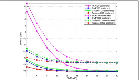
Fig. 7RMSE comparison for different number of scatterers versus SNRs, by 500 Monte-Carlo trials

simulations for different number of scatterers are imple-mented. The SNR range is 3 ∼ 30 dB; the numbers of independent trialsLis set to 500. The RMSE curves are shown in Fig. 7, where the solid lines and dashed lines indicate the experimental scenarios for 20 scatterers and 100 scatterers, respectively.

The simulation results indicate that the proposed algo-rithm performs superiorly compared with the reference methods for both the cases about the small and large num-ber of scatterers. It can be seen that even if the SNR is low, the performances of sparse reconstruction schemes are more robust than conventional PFA method. As a result of the sensitivity to noise, the RMSE curve of PFA shows conspicuous precipitous variation as the SNR is less than 18 dB. Considering the classic matching pursuit meth-ods, since there are merely 2kmax atoms to be chosen in each iteration, CoSaMP runs faster than OMP for SAR imaging, which is indicated by the statistical results of the

Table 1Average running time of imaging algorithms versus different SNRs

Time (s) SNR=3 dB SNR=12 dB SNR=21 dB SNR=30 dB

PFA 0.01736 0.01658 0.01564 0.01279

OMP 498.83 459.18 458.61 450.89

CoSaMP 1.1292 1.0759 1.0303 0.9784

Proposed 0.03719 0.03332 0.03135 0.03005

computational cost in Section 5.2.2. However, the sim-ulation results for RMSE show that the performance of CoSaMP is slightly worse than OMP. As a consequence, the existing SAR imaging methods are always difficult to achieve both the high speed and large success ratio of recovery. In contrast, by exploiting the multi-linear block sparsity of targets, the proposed algorithm can gain satisfactory performances on the both aspects.

5.2.2 Computing resources requirement

This section investigates the requirements for computa-tional cost. The configuration of this part is the same as Section 5.1.1 and the evaluation is done in terms of CPU time. The statistical results of running time for the case of different SNRs are shown in Table 1.

For the case about different numbers of scatterers, set the configuration to be the same as Section 5.1.1. The statistical results of running time are shown in Table 2.

Table 2Average running time of imaging algorithms versus different numbers of scatterers (indicated byNs)

Time (s) Ns= 20 Ns= 50 Ns= 100 Ns= 150

PFA 0.01716 0.01832 0.02437 0.04121

OMP 519.67 525.62 537.96 568.34

CoSaMP 0.95787 0.96073 0.98114 1.2098

The statistical data of Tables 1 and 2 indicate that there exist noteworthy differences of computational cost among these algorithms. The fastest two algorithms are PFA and the proposed algorithm, followed by CoSaMP and OMP in sequence. Nevertheless, the PFA cannot provide robust performance, as the RMSE comparison in the previous section. On the other hand, although the classic matching pursuit methods have high-resolution performance, the requirements to computing resources are considerable, especially for OMP algorithm. In each iteration, OMP must match every atom, which results in a high time consumption. As a contrast, the proposed algorithm can obtain the optimal RMSE performance and achieve a run-ning speed faster one order of magnitude than CoSaMP, which makes it suitable for the real-time applications.

6 Conclusions

In a practical scenario, the block sparse distribution of targets is a common assumption for SAR imaging. Nev-ertheless, the existing methods seldom take advantage of such geometrical feature. In this paper, a Kronecker constrained spotlight SAR imaging algorithm based on tensor decomposition is developed, which exploits the block sparsity of the target scene. HOSVD modeling of the decoupling signal received is employed by introduc-ing a preprocessintroduc-ing scheme for dictionary construction. Then, a multi-linear sparse reconstruction algorithm is deduced to obtain the estimation of scatter coefficients. Since the proposed algorithm utilizes the structural infor-mation of targets, a more robust performance can be achieved for imaging quality. A group of numerical exper-iments based on practical measured data are presented to verify the effectiveness of the developed method. In addi-tion, the complexity analysis indicates that the algorithm reduces the demand for computational cost comparing with the classic matching pursuit methods. The statisti-cal results of simulations confirm the superiority of the present algorithm as well, which is vitally important in real-time applications of engineering technique.

Acknowledgements

This work was supported in part by the National Natural Science Foundation of China (NSFC) under Grant U1533125 and National Science and technology major project under Grant 2016ZX03001022. The authors would like to thank the anonymous reviewers for their valuable comments that significantly improved the quality of this paper.

Authors’ contributions

Y-FG conceived and verified the feasibility of SAR imaging by introducing tensor modeling and developed the multi-linear sparse target reconstruction algorithm based on tensor decomposition; Y-FG, X-CC, and YY performed the experiments; GG and QW contributed to the design of numerical simulations; Y-FG wrote this paper; X-CC, YY, Y-BZ, and GG checked the manuscript and contributed to the rearrangement of the materials. All authors read and approved the final manuscript.

Competing interests

The authors declare that they have no competing interests.

Publisher’s Note

Springer Nature remains neutral with regard to jurisdictional claims in published maps and institutional affiliations.

Author details

1_{School of Electronic Engineering, University of Electronic Science and}

Technology of China, No. 2006, Xiyuan Ave., West Hi-Tech Zone, Chengdu 611731, China.2_{College of Telecommunication and Information Engineering,}

Nanjing University of Posts and Telecommunications, 66 Xinmofan Road, Nanjing 210003, China.

Received: 27 December 2016 Accepted: 19 May 2017

References

1. JC Curlander, RN McDonough,Synthetic Aperture Radar: Systems and Signal Processing. (Wiley-Interscience, New York, 1991)

2. GC Walter, SG Ron, MM Ronald,Spotlight Synthetic Aperture Radar. (Artech House Publishers, Norwood, 1995)

3. G Franceschetti, R Lanari,Synthetic Aperture Radar Processing. (CRC press, Boca Raton, 1999)

4. A Marino,Synthetic Aperture Radar. (Springer, Berlin, 2012), pp. 9–27 5. M Soumekh,Synthetic Aperture Radar Signal Processing with MATLAB

Algorithms. (Wiley-Interscience, New York, 1999)

6. E Mason, IY Son, B Yazici, Passive synthetic aperture radar imaging using low-rank matrix recovery methods. IEEE J. Sel. Topic Signal Process.9(8), 1570–1582 (2015). doi:10.1109/JSTSP.2015.2465361

7. R Baraniuk, P Steeghs, in2007 IEEE Radar Conference. Compressive radar imaging (IEEE, Boston, 2007), pp. 128–133

8. L Zhang, Qiao Z-j, M Xing, Y Li, Z Bao, High-resolution isar imaging with sparse stepped-frequency waveforms. IEEE Trans. Geosci. Remote Sens.

49(11), 4630–4651 (2011)

9. L Zhang, Z-J Qiao, M-D Xing, J-L Sheng, R Guo, Z Bao, High-resolution isar imaging by exploiting sparse apertures. IEEE Trans. Antennas Propag.

60(2), 997–1008 (2012)

10. B Sun, Y Cao, J Chen, C Li, Z Qiao, Compressive sensing imaging for general synthetic aperture radar echo model based on Maxwell’s equations. EURASIP J. Adv. Signal Process.2014(1), 153 (2014). doi:10.1186/1687-6180-2014-153

11. G Li, Q Hou, S Xu, Z Chen, Multi-target simultaneous isar imaging based on compressed sensing. EURASIP J. Adv. Signal Process.2016(1), 27 (2016). doi:10.1186/s13634-016-0327-1

12. Z Zhang, Y Xu, J Yang, X Li, D Zhang, A survey of sparse representation: algorithms and applications. IEEE Access.3, 490–530 (2015). doi:10.1109/ACCESS.2015.2430359

13. B Chen, J Wang, H Zhao, N Zheng, JC Príncipe, Convergence of a fixed-point algorithm under maximum correntropy criterion. IEEE Signal Process. Lett.22(10), 1723–1727 (2015)

14. W Ma, H Qu, G Gui, L Xu, J Zhao, B Chen, Maximum correntropy criterion based sparse adaptive filtering algorithms for robust channel estimation under non-gaussian environments. J. Frankl. Inst.352(7), 2708–2727 (2015)

15. J Fang, Z Xu, B Zhang, W Hong, Y Wu, Fast compressed sensing SAR imaging based on approximated observation. IEEE J. Sel. Topic Appl. Earth Obs. Remote Sens.7(1), 352–363 (2014)

16. L Zhang, J Duan, Z-J Qiao, M-D Xing, Z Bao, Phase adjustment and ISAR imaging of maneuvering targets with sparse apertures. IEEE Trans. Aerosp. Electron. Syst.50(3), 1955–1973 (2014)

17. J Zhang, Y Ban, D Zhu, G Zhang, Random filtering structure-based compressive sensing radar. EURASIP J. Adv. Signal Process.2014(1), 94 (2014). doi:10.1186/1687-6180-2014-94

18. X Zhang, G Liao, S Zhu, D Yang, W Du, Efficient compressed sensing method for moving-target imaging by exploiting the geometry information of the defocused results. IEEE Geosci. Remote Sens. Lett.

12(3), 517–521 (2015)

19. X Cong, G Gui, X Li, G Wen, X Huang, Q Wan, Object-level sar imaging method with canonical scattering characterisation and

inter-subdictionary interferences mitigation. IET Radar Sonar Navig.10(4), 784–790 (2016)

20. L Zhang, H Wang, Qiao Z-j, Resolution enhancement for isar imaging via improved statistical compressive sensing. EURASIP J. Adv. Signal Process.

21. L Zhao, L Wang, G Bi, S Li, L Yang, H Zhang, Structured sparsity-driven autofocus algorithm for high-resolution radar imagery. Signal Process.

125, 376–388 (2016)

22. R Bro, Parafac. tutorial and applications. Chemometr. Intell. Lab. Syst.

38(2), 149–171 (1997)

23. ND Sidiropoulos, R Bro, GB Giannakis, Parallel factor analysis in sensor array processing. IEEE Trans. Signal Process.48(8), 2377–2388 (2000) 24. A Cichocki, D Mandic, L De Lathauwer, G Zhou, Q Zhao, C Caiafa, HA Phan, Tensor decompositions for signal processing applications: from two-way to multiway component analysis. IEEE Signal Process. Mag.

32(2), 145–163 (2015)

25. L-H Lim, P Comon, Multiarray signal processing: tensor decomposition meets compressed sensing. Comptes Rendus Mecanique.338(6), 311–320 (2010)

26. MF Duarte, YC Eldar, Structured compressed sensing: from theory to applications. IEEE Trans. Signal Process.59(9), 4053–4085 (2011) 27. ND Sidiropoulos, A Kyrillidis, Multi-way compressed sensing for sparse

low-rank tensors. IEEE Signal Process. Lett.19(11), 757–760 (2012) 28. CF Caiafa, A Cichocki, Multidimensional compressed sensing and their

applications. Wiley Interdiscip. Rev. Data Min. Knowl. Disc.3(6), 355–380 (2013). doi:10.1002/widm.1108

29. S Friedland, Q Li, D Schonfeld, Compressive sensing of sparse tensors. IEEE Trans. Image Process.23(10), 4438–4447 (2014).

doi:10.1109/TIP.2014.2348796

30. E Li, MJ Shafiee, F Kazemzadeh, A Wong, Sparse reconstruction of compressive sensing multi-spectral data using an inter-spectral multi-layered conditional random field model. IEEE Access.4, 5540–5554 (2016). doi:10.1109/ACCESS.2016.2598320

31. M Haardt, F Roemer, G Del Galdo, Higher-order SVD-based subspace estimation to improve the parameter estimation accuracy in

multidimensional harmonic retrieval problems. IEEE Trans. Signal Process.

56(7), 3198–3213 (2008)

32. F Roemer,Advanced algebraic concepts for efficient multi-channel signal processing. (PhD thesis, Ilmenau University of Technology, Ilmenau, 2013) 33. TG Kolda, BW Bader, Tensor decompositions and applications. SIAM Rev.

51(3), 455–500 (2009). doi:10.1137/07070111X

34. DH Vu,Advanced techniques for synthetic aperture radar image reconstruction. (PhD thesis, University of Florida, Gainesville, 2012) 35. W Xu, P Huang, Y Deng, Efficient sliding spotlight SAR raw signal

simulation of extended scenes. EURASIP J. Adv. Signal Process.2011(1), 52 (2011). doi:10.1186/1687-6180-2011-52

36. L Zhang, Li H-l, Qiao Z-j, Xing M-d, Z Bao, Integrating autofocus techniques with fast factorized back-projection for high-resolution spotlight SAR imaging. IEEE Geosci. Remote Sens. Lett.10(6), 1394–1398 (2013) 37. L Greengard, J Lee, Accelerating the nonuniform fast fourier transform.

SIAM Rev.46(3), 443–454 (2004)

38. JA Tropp, Greed is good: algorithmic results for sparse approximation. IEEE Trans. Inf. Theory.50(10), 2231–2242 (2004)

39. S Jokar, V Mehrmann, Sparse solutions to underdetermined Kronecker product systems. Linear Algebra Appl.431(12), 2437–2447 (2009) 40. S Jokar, in2010 44th Annual Conference on Information Sciences and

Systems (CISS). Sparse recovery and kronecker products, (2010), pp. 1–4. doi:10.1109/CISS.2010.5464722

41. YC Eldar, M Mishali, in2009 16th International Conference on Digital Signal Processing. Block sparsity and sampling over a union of subspaces, (2009), pp. 1–8. doi:10.1109/ICDSP.2009.5201211

42. YC Eldar, P Kuppinger, H Bolcskei, Block-sparse signals: uncertainty relations and efficient recovery. IEEE Trans. Signal Process.58(6), 3042–3054 (2010)

43. RG Baraniuk, V Cevher, MF Duarte, C Hegde, Model-based compressive sensing. IEEE Trans. Inf. Theory.56(4), 1982–2001 (2010)

44. YC Eldar, M Mishali, Robust recovery of signals from a structured union of subspaces. IEEE Trans. Inf. Theory.55(11), 5302–5316 (2009).

doi:10.1109/TIT.2009.2030471

45. MF Duarte, RG Baraniuk, Kronecker compressive sensing. IEEE Trans. Image Process.21(2), 494–504 (2012)

46. Y-F Gao, L Zou, Q Wan, A two-dimensional arrival angles estimation for l-shaped array based on tensor decomposition. AEU - Int. J. Electron. Commun.69(4), 736–744 (2015). doi:10.1016/j.aeue.2015.01.001 47. DL Donoho, et al., High-dimensional data analysis: the curses and

blessings of dimensionality. AMS Math Chall. Lect., 1–32 (2000)

48. IV Oseledets, EE Tyrtyshnikov, Breaking the curse of dimensionality, or how to use SVD in many dimensions. SIAM J. Sci. Comput.31(5), 3744–3759 (2009)

49. B Sun, H Gu, M Hu, Z Qiao, inSPIE Sensing Technology+ Applications. Compressive sensing for a general sar imaging model based on maxwell’s equations (International Society for Optics and Photonics, San Diego, 2015), pp. 948402–948402

50. Y Li, Y Wang, Sparse SM-NLMS algorithm based on correntropy criterion. Electron. Lett.52(17), 1461–1463 (2016)

51. Y Li, C Zhang, S Wang, Low-complexity non-uniform penalized affine projection algorithm for sparse system identification. Circ. Syst. Signal Process.35(5), 1611–1624 (2016)

52. L De Lathauwer, B De Moor, J Vandewalle, On the best 1 and rank-(r 1, r 2,. . . , rn) approximation of higher-order tensors. SIAM J. Matrix Anal. Appl.21(4), 1324–1342 (2000)

53. R Rubinstein, M Zibulevsky, M Elad, Efficient implementation of the K-SVD algorithm using batch orthogonal matching pursuit. Technical Report 8, Computer Science Department, Technion - Israel Institute of Technology (2008)

54. JA Tropp, SJ Wright, Computational methods for sparse solution of linear inverse problems. Proc. IEEE.98(6), 948–958 (2010)

55. Y Yuan, J Sun, S Mao, PFA algorithm for airborne spotlight SAR imaging with nonideal motions. IEE Proc. Radar Sonar Navig.149(4), 174–182 (2002)

56. BD Rigling, RL Moses, Polar format algorithm for bistatic SAR. IEEE Trans. Aerosp. Electron. Syst.40(4), 1147–1159 (2004)