Dynamic tsunami generation due to sea-bottom deformation: Analytical
representation based on linear potential theory
Tatsuhiko Saito
National Research Institute for Earth Science and Disaster Prevention, Tsukuba, Ibaraki, Japan
(Received April 26, 2013; Revised June 13, 2013; Accepted July 16, 2013; Online published December 6, 2013)
Recording ocean-bottom pressures in offshore regions has increased our understanding of tsunami sources and promoted the development of rapid source estimation for early tsunami warning. Analytical solutions for the water height at the surface have often played an important role as a reference model in these efforts. To understand the system better and to develop the techniques further, not only the water height but the velocity in the sea and the pressure at the sea bottom are important. The present study obtains a solution for the velocity potential for sea-bottom deformation with an arbitrary source time function, and derives analytical solutions for the velocity distributions in the sea and the pressure at the bottom. These enable us to visualize the tsunami generation process, including the velocity field. The solutions can also give a theoretical background for setting the initial conditions of height and velocity in 2-D tsunami propagation simulations. Furthermore, the solution of the ocean-bottom pressure indicates that when the sea-bottom uplifts at an increasing rate, the sea-bottom pressure increases through a dynamic effect. This dynamic contribution will not be negligible as we develop more rapid and precise source estimation techniques using ocean-bottom pressure gauges within the source region.
Key words:Tsunami, theory, generation and propagation.
1.
Introduction
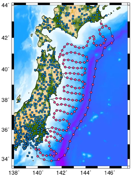
The tsunami generation/propagation problem has been a core focus of tsunami research. Laboratory experiments can accurately control the size and duration of the tsunami source and can observe the generation and propagation pro-cesses in situ, which is very useful for studying the funda-mental fluid dynamics of tsunamis (e.g., Hammack, 1973). Since a limited number of observation stations exist in the vast ocean, and tsunamis are usually recorded at sta-tions far from the source region, waveforms observed in-side the source region are rarely analyzed, and the nature of tsunamis are difficult to determine in detail. On 11 March, 2011, a hugeMW9.1 earthquake, known as the 2011 Tohoku-Oki earthquake, occurred off the Pacific coast of northeastern Honshu, Japan, where numerous sensors, such as seismometers, GPS stations, thermometers, and pressure gauges, were deployed (e.g., Itoet al., 2011; Sato et al., 2011). By analyzing the tsunami waveforms, in particu-lar, those recorded inside the source region, Saito et al. (2011) estimated the tsunami source with high resolution. Also, after the 2011 Tohoku-Oki earthquake, the National Research Institute for Earth Science and Disaster Preven-tion (NIED) started to construct a dense ocean-bottom net-work in and around the source region of the Tohoku earth-quake (Fig. 1) in order to detect seismic and tsunami signals more rapidly, and to contribute to more reliable seismic and tsunami warnings in the case of future gigantic earthquakes
Copyright cThe Society of Geomagnetism and Earth, Planetary and Space Sci-ences (SGEPSS); The Seismological Society of Japan; The Volcanological Society of Japan; The Geodetic Society of Japan; The Japanese Society for Planetary Sci-ences; TERRAPUB.
doi:10.5047/eps.2013.07.004
(e.g. Kanazawa and Shinohara, 2009; Monastersky, 2012; Uehira et al., 2012; Kanazawa, 2013). In order to fully interpret nearfield tsunami records or the sea-bottom pres-sure within the source region, theoretical models that can correctly include the tsunami generation process are very important.
Numerical simulation using a high-performance com-puter offers a method for theoretically calculating tsunami generation and propagation (e.g., Mader, 2004). Two-dimensional numerical simulation, using linear long-wave, linear dispersive, or non-linear tsunami equations, is a good choice for proper tsunami-propagation modeling (e.g., Shuto, 1991; Liu, 2009; Cuiet al., 2010; Saitoet al., 2010). Three-dimensional simulation is suitable when investigat-ing tsunami generation due to sea-bottom deformation, be-cause it is necessary to correctly simulate the vertical flow over the sea depth (Ohmachiet al., 2001; Grilliet al., 2002; Kakinuma and Akiyama, 2006). Saito and Furumura (2009) investigated tsunami generation due to sea-bottom defor-mation by numerically solving the 3-D equations of mo-tion. Nosov and Kolesov (2007) considered the compress-ibility of the fluid and synthesized the sea-bottom pressure records for the 2003 Tokachi-Oki earthquake. Maeda and Furumura (2013) developed a code in a framework of 3-D elastic equations of motion, which naturally simulates both seismic and tsunami waves, including their coupling effects. Dutykh et al.(2013) investigated the spatial and temporal distribution of water height during tsunami gener-ation based on linear and nonlinear theories.
In order to confirm the validity of the numerical simu-lations, and to interpret complicated simulated or observed waveforms, analytical solutions provide a good reference.
Fig. 1. Dense ocean-bottom seismic and tsunami stations (indicated by circles) are being constructed off the Pacific coast of northeastern Hon-shu, Japan (e.g. Uehiraet al., 2012; Kanazawa, 2013) and dense seismic stations (indicated by squares) are being operated on land (Okadaet al., 2004; Obaraet al., 2005) by the National Research Institute for Earth Science and Disaster Prevention (NIED).
The linear theory has been developed as a fundamental theory related to the generation/propagation problem (e.g., Lamb, 1932; Takahashi, 1942; Stoker, 1958; Leblond and Mysak, 1978; Mei, 1989; Ward, 2001). Using linear poten-tial theory, in which the velocity potenpoten-tial is introduced and wave linearity is assumed, the spatial and temporal change of the surface height due to bottom deformation are well reproduced in many instances, as observed in laboratory experiments and calculated in numerical simulations (e.g., Hammack, 1973; Kervella et al., 2007). One of the no-table consequences of the theory is that the height distri-bution at the surface is not always identical to the bottom deformation (e.g., Kajiura, 1963; Ward, 2001). Some stud-ies take this difference into account in order to calculate an initial tsunami-height distribution for 2-D tsunami propa-gation simulations (e.g., Tanioka and Seno, 2001). Saito and Furumura (2009) interpreted the relationship between sea-bottom deformation and the initial tsunami-height dis-tribution as two spatial lowpass-filter processes, in which the cut-off wavenumbers are given by the sea depth and the source duration. By taking these effects into account, and using the analytical solution for the water height, Tsushima et al.(2012) carefully investigated the ocean-bottom pres-sure records within the source region. In many past studies, the excess pressure at the sea bottom due to a tsunami is usually assumed to be given by a static contribution from the tsunami height; for instance, given byρ0g0η, whereρ0
is the density of sea water,g0is the gravitational constant, andηis the tsunami height. However, this approximation is not always valid. It is important to show the quantitative relationship, or the difference between tsunami height and the pressure at the bottom for more rigorous analyses.
Theoretical studies on tsunami generation have focused mainly on the water height at the surface (e.g. Kajiura, 1963; Dutykh, 2013). Few studies have investigated the ve-locity or displacement field in the sea during the tsunami generation. An exception was Ward (unpublished doc-ument available at http://es.ucsc.edu/˜ward/papers/Basic Tsunami Theory.doc), in which the solution of the displace-ment in the sea was theoretically derived for instantaneous sea-bottom uplift. Previous studies have the limitation that the mathematical expression of the velocity potential in the time domain has not yet been obtained for a sea-bottom de-formation characterized by an arbitrary source time func-tion. The solution has only been obtained through a formal expression using an inverse Fourier/Laplace transform, or for very limited situations. Dutykh and Dias (2007) and Kervellaet al.(2007) theoretically derived the velocity dis-tribution only at the sea surface, but not over the sea depth. They also derived the pressure at the sea bottom, but only after an instantaneous sea-bottom deformation. Levin and Nosov (2009) indicate the velocity potential in the time do-main for a very special case of the 1-D sea-bottom defor-mation characterized by constant-velocity uplift.
The velocity potential distribution in the sea is critically important in order to fully understand the generation pro-cess. Also, the sea-bottom pressure during tsunami gener-ation is critically important for developing a tsunami early warning because the sea-bottom pressure, rather than the water height, is currently measurable inside the source re-gion (e.g., Tsushimaet al., 2012). However, analytical so-lutions for the velocity in the sea and the pressure at the sea bottom have not yet been completed. This limitation comes from the fact that the velocity potential in the time domain has not generally been obtained.
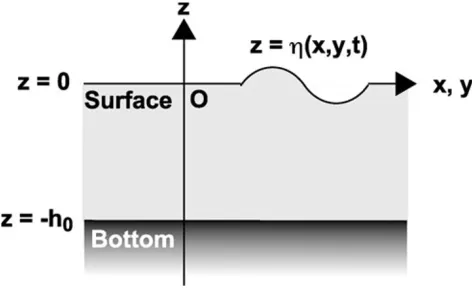
Fig. 2. Coordinates used for the formulation.
2.
Linear Potential Theory
2.1 A general frameworkWe formulate tsunami generation and propagation from sea-bottom deformation in a constant water depth based on linear potential theory (e.g., Takahashi, 1942; Hammack, 1973). We use the Cartesian coordinates shown in Fig. 2, where the z-axis is vertically upward, and the x- and y-axes lie in a horizontal plane. The sea surface is located atz=0, and the sea bottom is flat and located atz= −h0. We assume that the height of the sea surface η (x,y,t) at timet is small enough compared with the water depth
|η| h0, and viscosity is neglected. The velocity in the fluid is given by a vectorv (x,t) = vxex +vyey+vzez, wherex = xex +yey +zez, and ex, ey, and ez are the basis vectors in thex-,y-, andz-axes, respectively. We also assume an incompressible and irrotational flow,∇·v=0, in which the velocity vector is given asv(x,t)=gradϕ (x,t) using a velocity potentialϕ (x,t).
The velocity potential satisfies the Laplace equation
ϕ (x,t)=0, (1)
and the boundary conditions at the surface (z=0) are given by
∂ϕ (x,t)
∂t
z=0
+g0η (x,y,t)=0, (2)
∂ϕ (x,t)
∂z
z=0
−∂η (x∂,y,t)
t =0, (3)
where g0 is the gravitational constant. Equation (2) is a linearized dynamic boundary condition indicating that the pressure is constant along the sea surface, and Eq. (3) is a linearized kinematic boundary condition indicating that the sea surface does not break during the motion (e.g. Lamb, 1932; Stoker, 1958). Assuming the final sea-bottom defor-mation, or the permanent vertical displacement at the sea bottom, to be d(x,y), we give the vertical component of the velocity as the boundary condition at the sea bottom, as follows:
vz(x,t)|z=−h0 =d(x,y) χ (t) , (4)
where the functionχ (t)depends only on time, and satisfies
the following:
∞
−∞χ (t)dt=1. (5)
The functionχ (t)has the dimension of the inverse of time, and is referred to hereinafter as the source time function. We obtained the velocity potential that satisfies (1), (2), (3), and (4) as follows (e.g., Saito and Furmura, 2009):
ϕ (x,t)= 1 2π
∞
−∞dωexp [−iωt]χ (ω)ˆ
× 1
(2π)2
∞
−∞
∞
−∞dkxdkyexp
i kxx+i kyy
×1
k
ω2sinhkz+g
0kcoshkz
ω2coshkh
0−g0ksinhkh0
˜
dkx,ky
,
(6)
wherek=
k2
x+k2y,χ (ω)ˆ is the Fourier transform in the time-frequency domain defined as follows:
ˆ
χ (ω)=
∞
−∞dτexp [iωτ]χ (τ), (7)
andd˜kx,ky
is the 2-D Fourier transform in the space-wavenumber domain defined as follows:
˜
dkx,ky
=
∞
−∞
∞
−∞d xd y d(x,y)
×exp−ikxx+kyy
. (8)
Equation (6) represents a formal expression of the ve-locity potential with the inverse Fourier transform with re-spect to the time-frequency domain. This was derived by Takahashi (1942) in cylindrical coordinates. Similar equa-tions were obtained by Kervellaet al.(2007) and Levin and Nosov (2009) for the Cartesian coordinates using the in-verse Laplace transform. It is necessary to integrate over the angular frequencyωin order to obtain a solution in the time domain. Takahashi (1942) and Kervellet al.(2007) calculated the integral for the sea surfacez=0, but not for an arbitrary depth,z. Levin and Nosov (2009) performed the inverse Laplace transform for the velocity potential for any depth z. However, they assumed a very special case for the boundary condition at the sea bottom given by a linearly-increasing 1-D sea-bottom deformation (equations (2.67) and (2.68) in Levin and Nosov (2009)). A solution for the integration over the angular frequencyωin Eq. (6) has not yet been obtained for the sea-bottom deformation generally given by Eq. (4). The main difficulty with re-spect to the integration is that the residue theorem is not applicable to the sea-bottom deformation given by the arbi-trary functionχ (t)orχ (t) =δ (t). In the following, we theoretically derive the solution in the time domain for the sea-bottom deformation given by the arbitrary function of
χ (t).
2.2 A solution for constant elevation speed within a time period
functionχ (t)is given by a constant within a time periodT,
The Fourier transform of Eq. (9) is given by:
ˆ
χ (ω)= 1
iωT (exp [iωT]−1) . (11)
By considering this source time function (11), we can use the residue theorem for integrating with respect toωin Eq. (6). Substituting Eq. (11) into Eq. (6) and recognizing that poles are located atω=0,±√g0ktanhkh0, we calculated
(Appendix A). Equation (13) represents the dispersion re-lation for water waves (e.g., Stoker, 1958) and the corre-sponding phase velocity is given by:
c= ω0
Introducing the following function:
ψ (x,t)≡ −1
we can rewrite Eq. (12) as follows:
ϕ (x,t)=ψ (x,t)−ψ (x,t−T)
T . (16)
Equations (15) and (16) give the solution of the velocity potential for tsunami generation propagation when the sea-bottom deformation is represented by Eqs. (4) and (9).
2.3 A general solution: impulse response
Assuming that the duration T in Eq. (16) approaches zero, we obtain the solution for instantaneous sea-bottom deformation, or for the impulse response of the source time function given byχ (t)=δ (t). The solution is obtained as
By convoluting an arbitrary functionχ (t) with Eq. (17), we now obtain the solution of the velocity potential with respect to the function generally given by Eq. (4) as follows:
ϕ (x,t)=
∞
−∞ϕimpulse(x,t−τ) χ (τ)dτ. (18) We can confirm that we obtain an equation equivalent to Eq. (12) if we substitute Eq. (9) into Eq. (18). Furthermore, if we assume thatd˜kx,ky
solution of the impulse response for the point source at the
Using Eq. (17), we obtain the horizontal components of the velocity fieldvH =vxex+vyey, the vertical component of the velocityvz, and the height of the sea surfaceη for an instantaneous sea-bottom deformation, or the velocity at the bottom is given by the delta function, vz(x,t)|z=−h0 =
where∇H is the gradient in the horizontal plane given by
∇H =∂/∂xex+∂/∂yey, andkHis the wavenumber vector in the horizontal plane given bykH =kxex +kyey. Here, we introduce the distribution functions of the horizontal and vertical components of the velocity, as follows:
fH(k,z,h0)=coshkz+tanhkh0sinhkz, (23)
fz(k,z,h0)=
sinhkz
tanhkh0 +coshkz. (24)
We discuss the meaning of these distribution functions (Eqs. (23) and (24)) together with the interpretations of Eqs. (20)
through (22) in a later section (3.3 Propagation process). We can confirm that Eqs. (20) through (22) satisfy∇ ·v=0 and the boundary conditions (Eqs. (2) through (4)).
Ward (unpublished document available at http://es.ucsc. edu/˜ward/papers/Basic Tsunami Theory.doc) obtained an equation for displacement (equation (5.3.10) in the doc-ument) for an instantaneous sea-bottom deformation, whereas we have derived an expression for velocity (Eqs. (20) and (21)) in this study with the source term given by the delta function. The representation using the delta func-tion is fundamentally important for investigating physical phenomena during tsunami generation. This enables us to discuss the initial velocity distribution in a 2-D numerical simulation (see Section 3.2: On the use of the depth filter or Kajiura’s equation) and the pressure change during tsunami generation (see Section 2.4: Pressure at the sea bottom dur-ing the tsunami generation), in particular, for an arbitrary source time function characterized by a finite source dura-tion.
Ocean-bottom pressure gauges are often used for record-ing tsunamis (e.g., Tanget al., 2009). The pressure in the ocean is given by the sum of the hydrostatic pressure and an excess pressure due to the tsunami, i.e., −ρ0g0z+ pe, where the excess pressure is given by the velocity poten-tial as pe= −ρ0∂ϕ/∂t. Using the velocity potential of Eq. (17), we obtain the excess pressure brought about at the sea bottom by the tsunami as follows:
pe(x,t)|z=−h0= −ρ0
for an impulse response. Equation (25) is similar, but not identical, to that obtained by Dutykh and Dias (2007) and Kervellaet al.(2007), who derived the pressure at the sea bottom after an instantaneous sea-bottom uplift. However, they did not consider a source term, so the pressure change during the source process time cannot be inclusive. On the other hand, Eq. (25) includes an additional term (the second term in brackets{· · · }in Eq. (25)) as a source term, which represents the contribution from a dynamic source process. We refer to this term as the dynamic source term hereinafter in this manuscript. Equation (25) indicates that the excess pressure due to the tsunami is not simply given by a static contribution from the tsunami height. Only when the wavelength is long enough compared with the water depthkh0 1 and the dynamic source term is neglected, can the excess pressure due to the tsunami be approximated by pe ≈ ρ0g0η. We investigate the contribution from the dynamic source term in the following.
2.4 Pressure at the sea bottom during tsunami genera-tion
im-portant role for a rapid source estimation in an early tsunami warning (Tsushimaet al., 2009, 2011, 2012). It is crucially important to provide a representation of the pressure at the sea bottom, in particular, for an arbitrary source of duration
χ (t). For the source given by (4), we obtain:
In the derivation of Eq. (26), integrating by part, we calcu-late the time derivative of the delta function in Eq. (25) as the time derivative of the source time function in Eq. (26). This dynamic source term leads to an increase in excess pressure at the sea bottom when the sea bottom uplifts at an increasing ratedχ/dt>0.
We roughly examine how the dynamic source term con-tributes to the total ocean-bottom pressure during tsunami generation. Considering a simple case where the source size is large enough, kh0 1, and focusing on tsunami generation, neglecting propagation, and simplifying the ex-pression as cos [ω0(t−τ)]→1, we approximate Eq. (26)
In addition, assuming that the sea bottom uplifts with a con-stantly increasing ratedχ/dt=α0(>0)during the source process time from 0 toT, andχ (t)= 0 whent >T, we further simplify the first term in the brackets in Eq. (27) as−∞t χ (τ)dτ = α0t2/2, which should be equal to 1 at t = T (i.e.α0 = 2/T2, and
t
−∞χ (τ)dτ =t2/T2when t<T). The second term (the dynamic source term) is then given by h0 t2/T2 increases with elapsed time, whereas the dynamic source term h0
g0
dχ(t) dt =
2h0
g0T2 is constant during the source process time 0 ≤ t ≤ T. The contribution from the dy-namic source term to the total sea-bottom pressure att =T is then given by 2h0
g0T2 1+ 2h0
g0T2
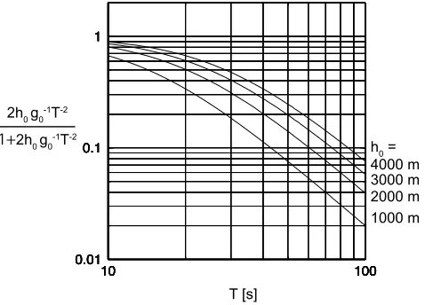
. The contribution from the dynamic source term increases as the sea depthh0 in-creases, and as the source process timeT decreases. Fig-ure 3 plots the contribution from the dynamic source term as a function of the source process time T, which indi-cates that the contribution from the dynamic source term can vary widely from 2% to 90% depending on the timeT and the sea depth. For example, supposing that the max-imum tsunami height occurred where the sea depth was
Fig. 3. Contribution of the dynamic source term to the total ocean-bottom pressure when the increasing rate is given by a positive constant. The contribution is plotted as a function of the source process timeT for various sea depths (h0=1000, 2000, 3000, and 4000 m).
∼3000 m and the corresponding rise time was ∼40 s as was the case in the 2011 Tohoku-Oki earthquake (Suzukiet al., 2011), we estimated that the dynamic source term con-tributes∼30%. Equations (25) and (26) should be used for more realistic situations, such as highly heterogeneous slip distributions and arbitrary source time functions (e.g. Geist, 2002). We can, at least, conclude that we cannot always ne-glect the dynamic source term. This is quite important for developing a rapid tsunami source estimation technique us-ing ocean-bottom pressure gauges inside the source region.
3.
Interpreting Tsunami Generation and
Propa-gation
3.1 Generation process
Fig. 4. Schematic illustrations of two tsunami problems. (a) Tsunami generation and propagation problem. Sea-bottom deformationd(x,y)generates an initial tsunami-height distribution, which we refer to herein as the generation process. The tsunami propagates from the initial tsunami-height distribution, which we refer to herein as the propagation process. (b) Tsunami propagation problem. The initial tsunami-height distributionη0(x,y) is given as an initial condition. This setting includes the propagation process, but not the generation process.
vH(x,t)= 1
(2π)2
∞
−∞
∞
−∞dkxdky
×expi kxx+i kyy
˜
η0
kx,ky
× −ig0kH ω0
fH(k,z,h0)sinω0t·H(t)
,
(29)
vz(x,t)= 1
(2π)2
∞
−∞
∞
−∞dkxdky
×expi kxx+i kyy
˜
η0
kx,ky
× {−ω0fz(k,z,h0)sinω0t·H(t)}, (30)
η (x,y,t)= 1
(2π)2
∞
−∞
∞
−∞dkxdkyexp
i kxx+i kyy
× ˜η0
kx,ky
cosω0t·H(t) , (31)
where η˜0
kx,ky
is the 2-D spatial Fourier transform of
η0(x,y).
Comparing Eqs. (20) through (22) and Eqs. (29) through (31), we recognize two differences. We may consider that the two points are peculiarities of the generation process. First,d˜kx,ky
/coshkh0appears in Eqs. (20) through (22) instead ofη˜0
kx,ky
as in Eqs. (29) through (31). The fac-tor 1/coshkh0has an effect that is sometimes referred to as a depth filter (e.g., Saito and Furumura, 2009; Tsushimaet al., 2012), and the corresponding equation in the spatial do-main is often referred to as Kajiura’s equation (e.g., Kajiura, 1963; Tanioka and Seno, 2001). This is a filtering effect from the sea bottom to the sea surface for an instantaneous sea-bottom deformation (e.g. Ward, 2001). The sea-bottom deformation in the wavenumber domain given byd˜kx,ky
is transmitted to the sea surface d˜kx,ky
/coshkh0 at a constant water depth ofh0 in the generation process (e.g. Takahashi, 1942; Ward, 2001; Dutykhet al., 2006; Dutykh and Dias, 2007; Kervellaet al., 2007).
Secondly, Eqs. (20) and (21) each have a term that in-cludes the delta function, whereas Eqs. (29) and (30) do not. These terms come from the term that includes the delta
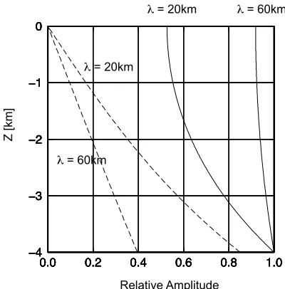
Fig. 5. Amplitudes of the source terms in the horizontal component (dashed lines) and the vertical component (solid lines) normalized by the vertical component at the sea bottom for values ofk=0.1 and 0.3 km−1, corresponding to wavelengthsλof 60 and 20 km for a water depth of 4 km (From Eqs. (20) and (21)).
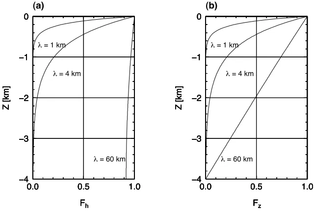
Fig. 6. Velocity distribution functions of (a) the horizontal component of the velocity (Eq. (23)), and (b) the vertical component of the velocity (Eq. (24)), plotted as functions of the depth,z, with a water depth ofh0 =4 km. The distribution functions forλ=1, 4, and 60 km (corresponding to k=6.28, 1.57, and 0.1 km−1, respectively) are plotted.
3.2 On the use of a depth filter or Kajiura’s equation
The initial tsunami-height distribution is not always equivalent to the sea-bottom deformation, particularly, for a steep sea-bottom deformation. In order to evaluate the ini-tial tsunami-height distribution from the sea-bottom defor-mation, Kajiura’s equation (e.g., Tanioka and Seno, 2001) or a depth filter (e.g., Tsushima et al., 2012) is used to make the correction. When using this corrected ini-tial tsunami-height distribution in 2-D numerical tsunami simulations, the initial velocity distribution is usually as-sumed to be zero. Ward (unpublished note available at http://es.ucsc.edu/˜ward/papers/Basic Tsunami Theory. doc) proved that a tsunami propagating from a bottom dis-placement is identical to one from the same initial tsunami-height distribution, except for the depth filter correction when the sea bottom uplifts instantaneously. We consider here an arbitrary source time function ofχ (t)and examine the initial conditions for 2-D numerical tsunami propaga-tion simulapropaga-tions using Eqs. (20) and (21).
Both Eqs. (20) and (21) appear to indicate that a non-zero velocity distribution exists due to both the first and the second terms in the brackets{· · · }. When considering the source time functionχ (t), Eq. (20) becomes
vH(x,t)= 1
(2π)2
∞
−∞
∞
−∞dkxdky
×expi kxx+i kyy
d˜kx,ky
coshkh0
× −ig0kH ω0
fH(k,z,h0)
×
t
−∞sin [ω0(t−τ)]
·χ (τ)dτ+ikH
k sinhkz·χ (t)
. (32)
Since the second term in Eq. (20) is represented by the delta
function, the second term becomes the source time function
χ (t) in Eq. (32). On one hand, the first term contains a function −∞t sin [ω0(t−τ)]χ (τ)dτ. When we assume that the source time functionχ (t)is non-zero only when t < T and is zero whent > T, the second term in the brackets{· · · }in Eq. (32) becomes zero and only the first term contributes to the velocity distribution whent >T. If we compare Eq. (32) with Eq. (29), we may suppose that the first term in the bracket{· · · }in Eq. (32) is generated from the water height distributiond˜kx,ky
/coshkh0. In other words, we may say that the velocity distribution fort >T is generated only through the water height distribution. Note that the same thing holds for the vertical flow (see Eq. (21)). Therefore, in order to properly include the tsunami gen-eration process in the initial tsunami height distribution for 2-D tsunami simulations, only the effect of the water height distribution (the first term in Eq. (32)) is taken into account at each time step of the tsunami simulation. We should not add the velocity distribution generated from the source. This procedure is the same as that usually used in past studies for 2-D tsunami simulations (e.g., Fujii and Satake, 2008; Saito and Furumura, 2009). Equation (32) is a funda-mental equation for validating the method for an arbitrary source time function.
3.3 Propagation process
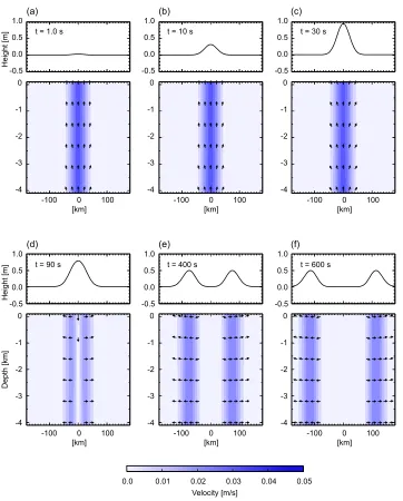
nor-Fig. 7. Surface height and velocity distribution for a large source (L = 2a = 60 km). The permanent sea-bottom deformation is given by
d0exp−x2/a2, whered0=1 m, and the source duration isT=31 s. The water height at the surface is shown in the upper panel, and the velocity distribution from the sea bottom to the sea surface is shown in the lower panel, for each elapsed timetfrom the start of sea-bottom deformation, (a)
t=1 s, (b) 10 s, (c) 30 s, (d) 90 s, (e) 400 s, and (f) 600 s. The vectors indicate the direction of the flow velocity in the fluid in the lower panel.
malized at the surface,z=0. Figure 6(a) graphs the distri-bution function of the horizontal component velocity (Eq. (23)) for values ofk =6.3, 1.6, and 0.1 km−1 correspond-ing to wavelengths of 1, 4, and 60 km for a water depth of 4 km. When the wavelength is small (λ = 1 km), the horizontal component of the velocity distributes only in the shallower regions (z<1 km). As the wavelength increases, the distribution function extends deeper. When the wave-length is much larger than the water depth (λ = 60 km
h0 = 4 km), the horizontal velocity component is dis-tributed almost uniformly over the entire depth. Figure 6(b) indicates the function for the vertical component velocity (Eq. (24)). As in the case of the horizontal components, when the wavelength is small (λ=1 km), the vertical com-ponent of the velocity is distributed only in the shallower region (z<1 km). Unlike the case of the horizontal com-ponents, when the wavelength is much larger than the water
depth (λ =60 km), the vertical component of the velocity does not distribute uniformly, but decreases with increasing depth, and the value becomes zero at the sea bottom. This indicates that the vertical velocity component is zero at the sea bottom for tsunami propagation.
4.
Examples
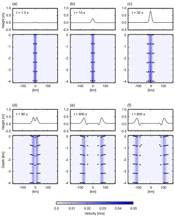
Fig. 8. Surface height and velocity distribution for a small source (L = 2a = 20 km). The permanent sea-bottom deformation is given by
d0exp−x2/a2, whered0=1 m, and the source duration isT=31 s. The water height at the surface is shown in the upper panel, and the velocity distribution from the sea bottom to the sea surface is shown in the lower panel, for each elapsed timetfrom the start of sea-bottom deformation, (a)
t=1 s, (b) 10 s, (c) 30 s, (d) 90 s, (e) 400 s, and (f) 600 s. The vectors indicate the direction of the flow velocity in the fluid in the lower panel.
As a simple example, we assume tsunami generation for a constant-rate sea-bottom deformation, the boundary con-dition of which is given by:
vz(x,t)|z=−h0 =d0exp
−x2
a2
· H(t)−H(t−T)
T . (33)
Substituting the corresponding Fourier transform of
˜
dkx,ky
= √πad0exp−a2k2x/4
· 2πδky
into Eqs. (20) through (22) and convoluting the corresponding source time function, we obtain the solution and plot the spatial and temporal water height and velocity distribution for the following two cases.
Large source
We consider the case in which the vertical component of the velocity at the sea bottom is given by Eq. (32)
with d0 = 1 m, a = 30 km, and T = 31 s. This
moves with a dominant horizontal flow (Figs. 7(e) and 7(f)). The horizontal velocity is always positive (negative) in hor-izontal locations where x is positive (negative). We see a small vertical component of the velocity near the surface, whereas no vertical component of the velocity exists near the bottom. The distribution functions (Fig. 6) also show these features when the wavelength is long (λ=60 km).
Small source
We then consider the case when a small source is given by L = 2a (=20 km) and T = 31 s (Fig. 8). During the source process time (T < 31 s), the vertical veloc-ity from the sea bottom produces a vertical flow of water over the source region (Figs. 8(a), 8(b), and 8(c)). How-ever, the maximum water height at the surface (0.8 m) is smaller than in the case of the larger source. This is in-terpreted that both the water depth and the source duration work as a kind of low-pass filter in space for the tsunami generation process (e.g., Saito and Furumura, 2009). Also, we may interpret this as showing that the vertical velocity is not efficiently excited by the excitation of the horizontal flow, for a small source such as is shown in Fig. 5. Af-ter the source process time ends (T > 31 s), the collapse of the uplifted sea surface accelerates, which causes a de-scending flow (Fig. 8(d)). The dede-scending water displaces the water sideways, and the water moves with a horizontal flow. Unlike the case of a large source, the vertical com-ponent of the velocity is also significant (Figs. 8(e) and 8(f)). The water height at the surface indicates a disper-sive wave. A short-wavelength tsunami propagates more slowly than a long-wavelength one. The horizontal compo-nent of the velocity distribution corresponding to the disper-sive wave oscillates between positive and negative values. Moreover, prograde-rotation of the velocity vector occurs near the surface. The velocity distribution accompanied by the short-wavelength tsunami is localized near the surface (Fig. 8(f)). This is consistent with the distribution functions for a short-wavelength case (Fig. 6). These phenomena re-lating to the dispersive wave are unique to deep waves or short-wavelength tsunamis.
5.
Concluding Remarks
We have presented a new solution for the velocity poten-tial in the time domain (Eqs. (17) and (18)) for an arbitrary sea-bottom deformation. Using this velocity potential, we can represent the spatial and temporal variation of the pres-sure at the sea bottom (Eq. (25)), the velocity distributions in the sea (Eqs. (20) and (21)), and the water height at the sea surface (Eq. (22)).
The solution for the ocean-bottom pressure (Eqs. (25) and (26)) indicates that when the sea bottom uplifts at an increasing rate, the sea-bottom pressure increases dynam-ically. This dynamic contribution will not be negligible as we develop more rapid and precise source estimation techniques using ocean-bottom pressure gauges within the source region (Figs. 1 and 3). The velocity distribution is represented by the sum of the direct and indirect com-ponents excited by the sea-bottom deformation (Eq. (32)): the direct component is the velocity distribution excited di-rectly by the sea-bottom deformation, while the indirect component is the velocity distribution excited by the
water-height distribution at the surface. The solution indicates that the direct component should be zero, or the initial ve-locity distribution should be zero at the initial conditions for 2-D tsunami propagation simulations. Using the solu-tions of Eqs. (20) through (22), we can visualize and inter-pret the spatial and temporal distributions of both the water height and the velocity vector in the sea from the sea-bottom deformation including, in particular, the finite duration of the source process time. We can interpret the generation and propagation using the amplitude distributions shown in Figs. 5 and 6.
The equations obtained in this study (Eqs. (17), (20) through (22), and (25)) are fundamental equations that con-stitute a mathematical basis for describing tsunami genera-tion and propagagenera-tion in incompressible water. These equa-tions enable us to interpret and analyze the records of the tsunami velocity field through the water and the records of the ocean-bottom pressure, whereas conventional equa-tions cannot. In particular, from the ocean-bottom pressure records within the source region, it is possible to extract in-formation relating to the acceleration of the sea-bottom de-formation, which is directly related to the dynamics of the earthquake fault rupturing. However, since actual records also contain acoustic waves (e.g. Yamamoto, 1982; Nosov and Kolesov, 2007; Maedaet al., 2011, 2013) that cannot be modeled by the incompressible theory assumed in this study, it is necessary to filter these out before applying the equations of the present study to the observed records. It is important to develop the equations for the case of com-pressible flow for future studies. Nevertheless, the analyt-ical solutions obtained herein can be used to validate sim-ulation codes because, at present, a number of numerical simulations assume an incompressible flow. Moreover, the solutions for an incompressible flow will serve as a sound basis for investigating the contribution of compressible flow in future studies.
Acknowledgments. The author would like to thank D. Inazu, T. Maeda, S. Ward, T. Hara, and an anonymous reviewer for careful reading and constructive comments.
Appendix A. Calculation of Eq. (12)
An artificial damping parameterε1 is introduced in Eq. (2) as:
∂ϕ (x,t)
∂t
z=0
+2ε1ϕ (x,t)
z=0
+g0η (x,y,t)=0,
(A.1)
and also another damping parameterε2in Eq. (9) as:
χ (t) = 1
T {H(t)−H(t−T)}exp(−ε2t) . (A.2)
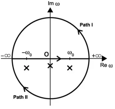
cor-Fig. A.1. Paths of the integral in the complexω-plane for Eq. (A.4). The poles (crosses) are located atω= −iε1±ω0and−iε2in the lower half plane.
responding to Eq. (12) is written as:
ϕ (x,t)= 1
Considering that the artificial damping is very small, or that the artificial damping parameters are much smaller than the angular frequency for tsunami, we employ the residue theorem. The poles of Eq. (A.3) are located atω= −iε1±
ω0 and−iε2 in the lower half of the ω-plane (Fig. A.1), whereω0=
√
g0ktanhkh0(see Eq. (13)). Whent−T <0, we take the path of the integral in the upper half plane (path I in Fig. A.1) including no poles. Whent−T >0, we take the integral path in the lower half plane including the poles (path II in Fig. A.1). The second term in the bracket in Eq.
(A.3), for example, is then calculated as:
∞
In a similar way, the first term in the bracket in Eq. (A.3) can also be calculated. The velocity potential (A.3) is then given by:
If Eq. (13) is used, Eq. (A.5) is confirmed to be identical to Eq. (12).
References
Cui, H., J. D. Pietrzak, and G. S. Stelling, A finite volume analogue of the PNC
1 -P1finite element: With accurate flooding and drying,Ocean Modeling,35, 16–30, doi:10.1016/j.ocemod.2010.06.001, 2010. Dutykh, D. and F. Dias, Water waves generated by a moving bottom, in
Tsunami and Nonlinear Waves, edited by A. Kundu, Springer Verlag, 2007.
Dutykh, D., F. Dias, and Y. Kervella, Linear theory of wave generation by a moving bottom,C. R. Acad. Sci. Paris, Ser. I,343, 499–504, 2006. Dutykh, D., D. Mitsotakis, X. Gardeil, and F. Dias, On the use of the finite
fault solution for tsunami generation problems,Theor. Comput. Fluid Dyn.,27, 177–199, 2013.
Fujii, Y. and K. Satake, Tsunami sources of the November 2006 and Jan-uary 2007 great Kuril earthquakes,Bull. Seismol. Soc. Am.,98, 1559– 1571, doi:10.1785/0120070221, 2008.
Geist, E. L., Complex earthquake rupture and local tsunamis,J. Geophys. Res.,107, doi:10.1029/2000JB000139, 2002.
Grilli, S. T., S. Vogelmann, and P. Watts, Development of a 3D numerical wave tank for modeling tsunami generation by underwater landslides,
Eng. Anal. Bound. Elem.,26, 301–313, 2002.
Hammack, J. L., A note on tsunamis: Their generation and propagation in an ocean of uniform depth,J. Fluid Mech.,60, 769–799, 1973. Ito, Y., T. Tsuji, Y. Osada, M. Kido, D. Inazu, Y. Hayashi, H. Tsushima,
region of the 2011 Tohoku-Oki earthquake, Geophys. Res. Lett., doi:10.1029/2011GL048355, 2011.
Kajiura, K., The leading wave of a tsunami,Bull. Earthq. Res. Inst.,41, 545–571, 1963.
Kakinuma, T. and M. Akiyama, Numerical analysis of tsunami generation due to seabed deformation,Doboku Gakkai Ronbunshuu B,62, 388– 405, 2006 (in Japanese with English abstract).
Kanazawa, T., Japan Trench earthquake and tsunami monitoring network of cable-linked 153 ocean bottom observatories and its impact to earth disaster science (UT2013-1147), International Symposium on Under-water Technology 2013, 2013.
Kanazawa, T. and M. Shinohara, A new, compact ocean bottom cabled seismometer system—Development of compact cabled seismometers for seafloor observation and a description of first installation plan,Sea Technology,50(7), 37–40, 2009.
Kervella, Y., D. Dutykh, and F. Dias, Comparison between three-dimensional linear and nonlinear tsunami generation models,Theor. Comput. Fluid Dyn.,21, 245–269, 2007.
Lamb, H.,Hydrodynamics, 6th ed., Dover Publications, 1932. Leblond, P. H. and L. A. Mysak,Waves in the Ocean, Elsevier, 1978. Levin, B. W. and M. A. Nosov,Physics of Tsunamis, Springer, 2009. Liu, P. L.-F., Tsunami modeling—propagation, inThe Sea, edited by A.
R. Robinson and E. N. Bernard, pp. 295–319, Harvard University Press, Cambridge, Massachusetts, 2009.
Mader, C. L., Numerical Modeling of Water Waves, CRC Press, Boca Raton, N. Y, 2004.
Maeda, T. and T. Furumura, FDM simulation of seismic waves, ocean acoustic waves, and tsunamis based on tsunami-coupled equations of motion,Pure Appl. Geophys.,170(1–2), 109–127, doi:10.1007/s00024-011-0430-z, 2013.
Maeda, T., T. Furumura, S. Sakai, and M. Shinohara, Significant tsunami observed at ocean-bottom pressure gauges during the 2011 off the Pacific coast of Tohoku Earthquake,Earth Planets Space,63, doi:10.5047/eps.2011.06.005, 2011.
Maeda, T., T. Furumura, S. Noguchi, S. Takemura, S. Sakai, M. Shinohara, K. Iwai, and S.-J. Lee, Seismic- and tsunami-wave propagation of the 2011 Off the Pacific Coast of Tohoku Earthquake as inferred from the tsunami-coupled finite-difference simulation,Bull. Seismol. Soc. Am.,
103(2B), 1456–1472, doi:10.1785/0120120118, 2013.
Mei, C. C.,The Applied Dynamics of Ocean Surface Waves, World Scien-tific Publishing Co. Pte. Ltd., 1989.
Monastersky, R., The next wave, Nature, 483, 144–146, doi:10.1038/483144a, 2012.
Nosov, M. A. and S. V. Kolesov, Elastic oscillations of water column in the 2003 Tokachi-oki tsunami source: In-situ measurements and 3-D numerical modeling, Nat. Haz. Earth Syst. Sci., 7, 243–249, doi:10.5194/nhess-7-243-2007, 2007.
Obara, K., K. Kasahara, S. Hori, and Y. Okada, A densely distributed high-sensitivity seismograph network in Japan: Hi-net by National Research Institute for Earth Science and Disaster Prevention,Rev. Sci. Instrum.,
76, 021301, doi:10.1063/l.1854197, 2005.
Ohmachi, T., H. Tsukiyama, and H. Matsumoto, Simulation of tsunami induced by dynamic displacement of seabed due to seismic faulting,
Bull. Seismol. Soc. Am.,91, 1898–1909, 2001.
Okada, Y., K. Kasahara, S. Hori, K. Obara, S. Sekiguchi, H. Fujiwara, and A. Yamamoto, Recent progress of seismic observation networks in
Japan—Hi-net, F-net, K-NET, and KiK-net,Earth Planets Space,56, xv–xxviii, 2004.
Saito, T. and T. Furumura, Three-dimensional tsunami generation simu-lation due to sea-bottom deformation and its interpretation based on the linear theory,Geophys. J. Int.,178, 877–888, doi:10.1111/j.1365-246X.2009.04206.x, 2009.
Saito, T., K. Satake, and T. Furumura, Tsunami waveform inversion includ-ing dispersive waves: The 2004 earthquake off Kii Peninsula, Japan,J. Geophys. Res.,115, B06303, doi:10.1029/2009JB006884, 2010. Saito, T., Y. Ito, D. Inazu, and R. Hino, Tsunami source of the
2011 Tohoku-Oki earthquake, Japan: Inversion analysis based on dispersive tsunami simulations, Geophys. Res. Lett., 38, L00G19, doi:10.1029/2011GL049089, 2011.
Sato, M., T. Ishikawa, N. Ujihara, S. Yoshida, M. Fujita, M. Mochizuki, and A. Asada, Displacement above the hypocenter of the 2011 Tohokuk-Oki Earthquake, Science, 332, 1395, doi:10.1126/science.1207401, 2011.
Shuto, N., Numerical simulation of tsunamis—Its present and near future,
Nat. Hazards,4, 171–191, doi:10.1007/BF00162786, 1991.
Stoker, J. J.,Water Waves: The Mathematical Theory with Applications, John Wiley and Sons, Inc., 1958.
Suzuki, W., S. Aoi, H. Sekiguchi, and T. Kunugi, Rupture pro-cess of the 2011 Tohoku-Oki mega-thrust earthquake (M9.0) in-verted from strong-motion data, Geophys. Res. Lett., 38, L00G16, doi:10.1029/2011GL049136, 2011.
Takahashi, R., On seismic sea waves caused by deformations of the sea bottom,Bull. Earthq. Res. Inst.,20, 357–400, 1942 (in Japanese with English abstract).
Tang, L., V. V. Titov, and C. D. Chamberlin, Development, testing, and ap-plications of site-specific tsunami inundation models for real-time fore-casting,J. Geophys. Res.,114, C12025, doi:10.1029/2009JC005476, 2009.
Tanioka, Y. and T. Seno, Sediment effect on tsunami generation of the 1896 Sanriku tsunami earthquake,Geophys. Res. Lett.,28, 3389–3392, 2001. Tsushima, H., R. Hino, H. Fujimoto, Y. Tanioka, and F. Imamura, Near-field tsunami forecasting from cabled ocean bottom pressure data,J. Geophys. Res.,114, B06309, doi:10.1029/2008JB005988, 2009. Tsushima, H., K. Hirata, Y. Hayashi, Y. Tanioka, K. Kimura, S. Sakai, M.
Shinohara, T. Kanazawa, R. Hino, and K. Maeda, Near-field tsunami forecasting using offshore tsunami data from the 2011 off the Pacific coast of Tohoku Earthquake,Earth Planets Space,63, 821–826, 2011. Tsushima, H., R. Hino, Y. Tanioka, F. Imamura, and H. Fujimoto, Tsunami
waveform inversion incorporating permanent seafloor deformation and its application to tsunami forecasting,J. Geophys. Res.,117, B03311, doi:10.1029/2011JB008877, 2012.
Uehira, K., T. Kanazawa, S. Noguchi, S. Aoi, T. Kunugi, T. Matsumoto, Y. Okada, S. Sekiguchi, K. Shiomi, and T. Yamada, Ocean bottom seis-mic and tsunami network along the Japan Trench, AGU Fall Meeting, OS41C-1736, 2012.
Ward, S. N., Tsunamis, in The Encyclopedia of Physical Science and Technology, edited by R. A. Meyers, Academic, San Diego, Calif, 2001. Yamamoto, T., Gravity waves and acoustic waves generated by submarine