R E V I E W
Open Access
Evaluation of a class of NLFM radar
signals
Sebastian Alphonse
*and Geoffrey A. Williamson
Abstract
Signal design is an important component for good performance of radar systems. Here, the problem of determining a good radar signal with the objective of minimizing autocorrelation sidelobes is addressed, and the first
comprehensive comparison of a range of signals proposed in the literature is conducted. The search is restricted to a set of nonlinear, frequency-modulated signals whose frequency function is monotonically nondecreasing and antisymmetric about the temporal midpoint. This set includes many signals designed for smaller sidelobes including our proposed odd polynomial frequency signal (OPFS) model and antisymmetric time exponentiated frequency modulated (ATEFM) signal model. The signal design is optimized based on autocorrelation sidelobe levels with constraints on the autocorrelation mainlobe width and leakage of energy outside the allowed bandwidth, and we compare our optimized design with the best signal found from parameterized signal model classes in the literature. The quality of the overall best such signal is assessed through comparison to performance of a large number of randomly generated signals from within the search space. From this analysis, it is found that the OPFS model proposed in this paper outperforms all other contenders for most combinations of the objective functions and is expected to be better than nearly all signals within the entire search set.
Keywords: Radar signal processing, Signal design, Matched filters, Frequency modulation, PSLR, ISLR
1 Introduction
Radar’s primary objective is to detect targets and estimate their range and velocity. To achieve these objectives, it is desirable that the radar signals have small autocorrela-tion (AC) sidelobes or Doppler tolerant. Optimizing over one characteristic can yield other undesired effects such as widening the AC mainlobe. Achieving a balance between the conflicting requirements is the goal of signal modu-lation. Radar signals are either frequency modulated or phase modulated. In this paper, we address finding FM signals that have high-quality performance on reducing the sidelobes with the constraints on mainlobe width and energy leakage beyond the specified bandwidth.
The most popular frequency modulation (FM) sig-nal is linear frequency modulation (LFM). Though LFM has good Doppler tolerant characteristic, it has relatively
high sidelobes (− 13.4 dB) which may not be suited
for many other radar applications. To achive smaller
*Correspondence:salphons@hawk.iit.edu
Department of Electrical and Computer Engineering, Illinois Institute of Technology, Chicago, IL, 60616, USA
AC sidelobes and also to maintain constant envelope, researchers turned to stationary phase principle (SPP) in which the frequency function is varied nonlinearly to shape the PSD to one that corresponds to smaller AC sidelobes.
Using this principle, Cook [1] derived frequency
func-tions whose PSDs have the shape of an nth power of
cosine. Cook also noted that deriving the frequency func-tion from the PSDs can be done only for relatively sim-ple PSDs, and in his paper [1], Cook derived frequency functions only forn = 1, 2, 3, and 4. The best peak
side-lobe level he reported was of − 47dB for the choice of
n = 4. The limitation of SPP to use only simple PSDs
led researchers to come up with ad hoc frequency func-tions that have desirable PSDs resulting in smaller AC sidelobes. In 1979, Price proposed a nonlinear frequency function that achieves small sidelobes [2], ([3], Section 5.2), ([4], Section 8.2.2). After Price’s nonlinear frequency modulation (NLFM), many researchers proposed ad hoc frequency functions with the aim of achieving smaller AC sidelobes [5–9]. These NLFM signals are from the sig-nal set: these signals have monotonically increasing and
midpoint antisymmetric frequency functions. These fre-quency functions have a continuously varying first deriva-tive, except for specific parameter settings in which case they result in LFM.
There is another class of NLFM signals that also belongs
to the signal set but whose frequency functions have
three segments [10–13]. In the middle segment, the
frequency is a linear function of time having constant first derivative. The first and the third segments have derivatives diverging from this particular constant value.
Cook [10] proposed such an NLFM signal whose
fre-quency function has three piecewise linear components and achieved a peak sidelobe level below−30 dB. Though in this case the first and third components are linear, Cook suggested that these components can be nonlin-ear. Griffiths and Vinagre [11] used this piecewise linear FM signal and applied amplitude modulation to get fur-ther reduction in sidelobe levels. Ofur-ther researchers sug-gested nonlinear functions for the first and third segments to achieve reduced sidelobe levels without performing amplitude modulation [12,13].
1.1 Objective functions
We are interested to find the “best” NLFM signal with small sidelobes. To do this, we define a family of objective functions that penalize AC sidelobes. The AC of signalsis defined as
Rs(m)=
M−m−1
n=0 s(n+m)s∗(n), m≥ 0,
R∗s(−m), m<0. (1)
The papers we have discussed so far focus on minimiz-ing only peak sidelobe level with respect to the mainlobe level. Another important performance metric often con-sidered in the literature is the integrated sidelobe ratio (ISLR), which is the energy in sidelobes with respect to the energy in the mainlobe [14–16]. It is reasonable to form objective functions that are convex combinations of ISLR and the peak-to-sidelobe ratio (PSLR). By choosing the convex weighting between zero to one, the radar operator can emphasize one metric over the other.
PSLR is defined as the ratio of maximum sidelobe level squared with respect to the mainlobe level squared. If we denote thepth AC sidelobe peak value asRp, then
PSLR(s)=
There are few slightly varying definitions for ISLR used in the literature. The one we have used in this paper is the one that is widely used [15,17,18] in which, the ISLR is defined as the ratio of energy in the AC when the signals are not time aligned to the energy in AC when the signals are time aligned. In this case, one sample correspond to one sample delay in autocorrelation function.
ISLR(s)=
A signal with small sidelobes will have smaller values for both PSLR and ISLR. We form a cost function as the convex combination of these two metrics. Note that PSLR is always less than one and ISLR can be greater than one depending on the signal model. This will force the optimization procedure to give more importance in minimizing ISLR. To bring both these objectives to a comparable level, we will normalize PSLR and ISLR with respect to LFM’s PSLR and ISLR:
NPSLR(s)= PSLR(s)
PSLRLFMand ISLRLFM are the PSLR and ISLR of the
LFM signal whose frequency is a linear function of time. Hence, our cost function to minimize is
Q(s;β)=β·NPSLR(s)+(1−β)·NISLR(s), (6)
whereβ∈[0, 1] is a weight parameter.
While minimizing PSLR and ISLR, the radar designer also considers the AC mainlobe width and amount of transmitted signal energy contained in the allowed band-width. Reducing the sidelobe level widens the mainlobe. Though reducing the sidelobes is a higher priority, hav-ing a very wide mainlobe reduces the range accuracy of the target [19]. Also. a wide AC mainlobe of a signal reflected from a strong target will mask the reflection from a weak target. Hence, we will impose a constraint that the AC mainlobe width of the signal (MLW(s)) should not be larger than twice the mainlobe width of LFM (MLW(s)/MLWLFM ≤ 2), and we optimizeQ(s;β)in (6)
subject to this constraint.
bandwidthB0. To quantify the signal’s spectral occupancy,
we will define in-band energy ratio (IBER) as
IBER(s)= Energy ofsin the spectral range [−B0/2,B0/2]
Total energy of the signals .
(7)
In this paper, we will limit our search for the best signal within the set whose signals have at least 90% of the signal
energy within the specified bandwidth (IBER ≥ 0.9). It
should be noted that the mainlobe width factor (two) and IBER (0.9) depend on the particular applications and the choices we have made in this paper fall under a reasonable range of values for these parameters.
1.2 Related work on finding good FM signals with small sidelobes
When the radar operator chooses a signal for his objective, it is useful to have a performance comparison of available radar signal designs. Though many papers have proposed different NLFM signal models, there has been little focus on comparing these signal models. Boukeffa et al. [22] compares different NLFM signal models, but there are some discrepancies in the results. For example, according to [22], the peak sidelobe level for Cook’s [1] proposed sig-nal whose PSD has the shape of cosine to the power four is−84 dB. But Cook himself reported the peak sidelobe level as−47 dB. It is not clear from these papers, how they obtained these values. We used 10 log10((PSLR(s)) (PSLR(s)from Eq. (2)), which is the common expression
for computing PSLR in decibel. Wenzhen and Yan [7]
compared several NLFM signal models (including Price’s signal model) along with their own proposed NLFM signal. Though in their comparison, their proposed signal model achieved smaller sidelobes, we observed from our analysis that Price’s signal model outperforms the signal model proposed in [7].
1.3 Our contribution
In this paper, we present the odd polynomial frequency signal (OPFS) and the asymmetric time exponentiated FM (ATEFM) signal. Polynomial-phase signals (PPS) are com-mon in radar applications. As the name suggests in PPS, the polynomial represents the phase of the signal. While designing NLFM, representing the frequency function as a polynomial gives direct control over the PSD which helps to reduce AC sidelobes. An important distinction of OPFS is that even powers to set zero due to the antisym-metric nature of the frequency functions from the signal set. Hence we reference this signal as odd polynomial frequency signal (OPFS).
From our experiments, we observed that extending the frequency function beyond the allowed bandwidth range
helps in reducing the AC sidelobe levels. In the proposed signal model, we incorporate a frequency scaling param-eter which helps in extending the frequency function beyond the allowed bandwidth range. Care must be taken to limit this extension to focus most of the signal energy within the allowed bandwidth. Through simulation, we will demonstrate that OPFS outperforms other signals for most of the weighted combinations of objective func-tions that we consider. And the signal proposed by Price [2] outperforms the other signals when only minimizing PSLR.
The best signal inmay not be from any of the param-eterized signal subsets that we studied. To assess the likelihood of a better signal within from outside the parameterized subsets we have considered, we examine randomly selected signals indrawn according to a uni-form probability distribution. In Section4, we discuss how we generate such signals. We created one million ran-dom signals and determined the best signal among them with respect to each choice of weights for the objective function. We observed that our 6D-OPFS and Price’s sig-nal still outperform these randomly picked sigsig-nals. From this experiment, as discussed in Section 4, we estimate with 95% confidence that 6D-OPFS and Price’s signal outperforms 99.9997% of the signals in.
2 Library of parameterized NLFM signals
The general form for radar signals is s(t) = A(t) expjφ(t), whereA(t)is the time dependent amplitude of the signal. A varying envelope of the signal reduces transmitter efficiency. In this paper, we will assume that the signals have constant amplitude (A(t)=A).φ(t)is the phase of the signal. Depending on the search range of the radar and desired range resolution, the radar signal is lim-ited to have a pulse durationT, bandwidthB, and carrier frequencyfc. It is easier to design the signal in baseband, and hence, without loss of generality, we will setfcto zero. The phase of the signalφ(t)can be written as an integral of the frequency function f(t). The frequency functions of the FM signals proposed in the literature for small sidelobes are nondecreasing and antisymmetric about the temporal midpoint, and we restrict consideration to fre-quency functions of this form. The class of frefre-quency functions f(t) we consider thus satisfy the following conditions:
(A) f(−T/2)= −B/2.
(B) f(t)is monotonically nondecreasing. (C) f(−t)= −f(t).
Fig. 1Typical frequency function from the NLFM signal set, which is monotonically nondecreasing and has temporal midpoint antisymmetry
(defined in (7)), but care must be taken during design to make sure that the significant part of the signal energy is contained within the useful bandwidth.
In Fig.1, we show an example of a frequency function
from the signal set that typifies the NLFM frequency
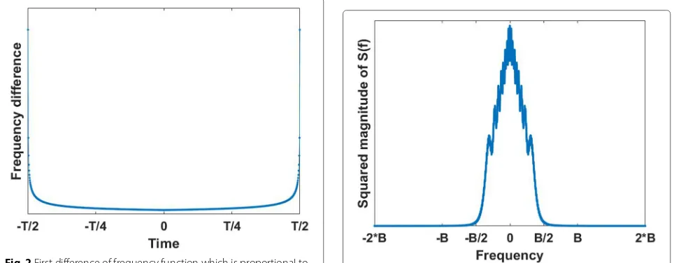
functions proposed in the literature designed for smaller sidelobes. By studying the frequency characteristics of this typical signal, we can understand why the signals from the signal set yield smaller sidelobes. The first difference which is proportional to first order derivative of this typ-ical frequency function with respect to time is shown in
Fig. 2First difference of frequency function which is proportional to the first derivative of the typical frequency function shown in Fig.1. The derivative has large value near the start and stop of the signal which correspond to the frequency band edges and small value at the low frequencies (from baseband perspective). Hence, as per SPP, the signal spends small time at the band edges and more time at the center frequencies
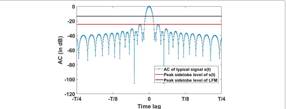
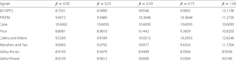
Fig.2. We can observe that a typical frequency function has high derivative at the start and end of the signal. The spectral energy at the edges of the frequency band arises from these fast variations at the start and end of the signal. Moreover, the frequency function has a small derivative in the temporal middle of the signal duration, corresponding to the low frequencies (from a baseband perspective). This means the frequency function spends less time in the edge frequencies and more time in the low frequencies. As per the SPP, this results in smaller energy in edge frequencies and higher energy in the low frequencies as we can see in Fig.3. As a result, we get a windowed PSD which yields smaller AC sidelobes as shown in Fig.4. We can observe that the red (lower) horizontal line in Fig. 4 is the peak sidelobe level of this typical NLFM signal which is sub-stantially smaller compared to the peak sidelobe level of LFM shown as the black (upper) horizontal line.
Each of the NLFM signal models proposed in the
lit-erature is characterized by its own set of parameters
that determine the specific nonlinear characteristics of the frequency function. In this section, we discuss the two sig-nal models proposed by us the authors. The other sigsig-nal models that we have selected from the literature for com-parison are discussed inAppendixfor reference. We made minor modifications to the notations to be in consistent with our notations. We have selected what we feel are the most representative among the classes of NLFM signals designed for smaller sidelobes published in the literature. We label the sets of signal models as A, B,. . .,H. However, there are other signal models that we do not
Fig. 4AC of the typical frequency function shown in Fig.1. The red (lower) line shows the peak sidelobe level of the typical NLFM signal. The black (upper) line is the peak sidelobe level of LFM, which is significantly higher than that of NLFM
include here. Such signals can reasonably viewed as vari-ation [6] of the signals that we do include for comparison or the signal models that require more information to recreate [8,9] for comparison.
2.1 Odd polynomial frequency signal:A
Our proposed polynomial frequency function is
f(t) = ζB N
k=0
pk(2t/T)N−k,−T
2 ≤t≤
T
2. (8)
Since the frequency function in the signal set is
antisymmetric, we set the coefficients corresponding to the even powers pN,pN−2,pN−4,. . . to zero and
opti-mize the coefficients corresponding to the odd powers pN−1,pN−3,pN−5,. . .. Optimizing only the odd
coeffi-cients helps the optimization routines to focus only on the important parameters. Though higher degree poly-nomials can result in flexible frequency functions, we observed from our experiments the polynomial degree higher than 11 did not yield improvements in terms of AC characteristics. Eleventh degree polynomial has six odd coefficients and hence has six dimensional freedom. We refer this signal as 6D-OPFS. In this paper, we use the AC characteristics of 6D-OPFS to compare against other FM signal models. Though we intend most of the signal energy to be within the allowed bandwidth, we inten-tionally allow small amount signal energy to leak beyond the allowed band to have larger effective bandwidth. This can enhance the AC characteristics of the signal. The parameterζin (8) helps in extending the frequency func-tion beyond the allowed bandwidth range of [−B/2,B/2].
The parameter set for the 6D-OPFS is given byA =
{ζ,p1,p3,p5,p7,p9,p11}.
2.2 Asymmetric time exponentiated FM (ATEFM):B
The frequency function of ATEFM has a single parameter
Bwithν∈(1, 2] used to control the nonlinearity:
f(t,ν)= ⎧ ⎪ ⎨ ⎪ ⎩ B
2
2(t+T/2) T
ν−1 − B
2, −2T ≤ t <0,
B
2 −B2
2(T/2−t) T
ν−1
, 0≤ t < T2. (9)
This signal is used as an example in [23] to compute an accurate estimate of NLFM signals transmitted by non-cooperating radars at low SNRs.
3 Signal optimization
For the simulation study, we consider discrete time radar signals of the forms(t) = Aexpjφ(t), where the phase
φ(t) is the integral of the frequency function f(t) with sample time values att = nT/Mforn = 0, 1,. . .,M− 1. The signal’s AC characteristics depend on the
time-bandwidth productBT and not on the individual values
of pulse durationT and bandwidthB. From our simula-tion experiments, we observed that for different values of BTthe relative performance of the AC characteristics of the considered signal models remain the same. Here, we present the simulation results forBT = 100. We set the design parameters as follows.
1. Available signal bandwidth isB=10MHz and the pulse duration of the signal isT =10μs.
2. Number of samplesM=1001resulting in the sampling frequency ofFs=M/T =100.1MHz which conveniently satisfies the Nyquist condition with respect to the chosen signal bandwidthB.
From each of the parameterized signal sets A,
s∗#(β)=arg min s∈#0
Q(s;β) (10)
whereβis the weight parameter defined in Eq. (6) and # ∈
{A,B,C,D,E,F,G,H}. The signal set denoted byA0is
the subset of signals from the signal setAthat satisfy the AC mainlobe width and bandwidth requirements defined in Section 1.1. In a similar manner, we define the other parameterized signal subsetsB0, C0,. . .,H0.s∗A(β)as the best signal from the signal set A0 with respect to
the cost functionQ(s;β). Similarly,s∗B(β)is the best signal from the parameterized signal setB0and so on. To find
these best signals s∗A(β), s∗B(β),. . .,s∗H(β) from each of the signal subsetsA0, B0,. . .,H0, we need to find the
optimum values for the parametersA, B,. . .,H. We used global optimization routines in Matlab [24] based on simulated annealing and pattern search methods to search for these optimum parameters from which we obtain the best signalss∗A(β), s∗B(β),. . .,s∗H(β).
For reference, Table 1 shows the signal parameters
obtained from the optimization routines for all the signal models. We have also listed the PSLR and ISLR obtained for all the signals using these optimum parameters in Table2and Table3. Figure5shows the summary of the cost valuesQ(s∗A,β),Q(sB∗,β),. . .,Q(s∗H,β)plotted versus
the cost function weightβ. We vary the weightβ from
0.00 to 1.00 in steps of 0.25. Note thatβ =0 corresponds
to minimizing only the ISLR and β = 1 corresponds
to minimizing only PSLR. We can observe that the 6D-OPFS signal outperforms the other signal models for all
the considered weights except whenβ = 1. Forβ = 1,
Price’s 6D-OPFS, Collins and Atkins, Wenzhen and Yan, and Cook’s signal designs have cost function close to zero (which can be observed in the last column of Table 2). In this case, Price’s signal models achieves the minimum cost.
4 Discussion on sub-optimality of s∗A(β),. . .,s∗H(β)and simulation results
In the preceding section, we found the best signals from within the parameterized signal setsA0,. . .,H0. Note
that these signal setsA0,. . .,H0are subsets of0. We
noticed the signal set 6D-OPFS (A0) and the signal set
proposed by Price (D0) outperform the other
parame-terized signal sets for the cost functions we considered. However, the best overall signal from the signal set 0
may not lie in any of A0,. . .,H0. In order to
char-acterize how good s∗A(β),. . .,s∗H(β) and particularly the optimal signalss∗A(β)ands∗D(β)are, we are interested to
Table 1Table listing signal parameters obtained from optimization routines forB=1000,T=0.1, andM=1001
Signals β=0.00 β=0.25 β=0.50 β=0.75 β=1.00
6D-OPFS ζ 1.2 1.4 0.9969788 1.4 1.0888194
p1 2.9833301 3.0322699 3.2706690 2.3061778 3.8595594 p3 −6.0137280 −5.7741939 −6.0897503 −4.5383562 −4.9449954 p5 4.4237943 4.1432707 3.8108525 3.1916240 1.7412935 p7 −1.3836515 −1.4752306 −0.7409933 −0.8812900 0.0453272 p9 0.1308622 0.3757097 0.0982280 0.1745349 0.3363182 p11 0.4617059 0.2827204 0.4160720 0.2849106 0.0630924
ATEFM ν 2.0957537 1.7356345 1.6155135 1.6155135 1.4533719
Cook n 1 4 4 4 4
Price Bl 0.8436638 0.6848811 0.5611050 0.4381695 0.1296791
Bc 0.1154728 0.1847406 0.2379900 0.2909956 0.3511787
Collins and Atkin α 2.79×10⁻⁷ 7.9176303 0.8057049 0.6119288 0.8456120
γ 5.22×10⁻⁵ 0.3160832 1.0382372 1.2681669 1.4259004
Wenzhen and Yan k1 0.3893824 0.3987516 0.3896719 0.2541758 0.1094573 k2 2.0355661 2.0105194 2.0347858 2.4453675 3.0024526
Vizitiu-Arcsin f 0.6324528 0.4586289 0.4500549 0.4297516 0.4243944 t 5.9713625 6.3463664 6.3915436 6.5225125 6.5638456
Vizitiu-Power f 0.5602052 0.3627173 0.2660381 0.2117072 0.2412588 t 6.0205251 6.1973325 5.6443412 5.0191368 5.4134402
Table 2PSLR of the parameterized signals computed with the parameters obtained from optimization routines
Signals β=0.00 β=0.25 β=0.50 β=0.75 β=1.00
6D-OPFS −14.6434 −25.4724 −33.7720 −33.2736 −51.7987
ATEFM −12.2009 −18.8418 −23.6508 −23.6508 −24.7634
Cook −21.6920 −34.4314 −34.4314 −34.4314 −34.4314
Price −19.7837 −24.3293 −28.8422 −34.3562 −59.5167
Collins and Atkins −13.4874 −21.2493 24.4017 −29.1210 −39.1003 Wenzhen and Yan −23.9121 −23.8514 −23.9103 −32.5355 −50.0584 Vizitiu-Arcsin −16.5711 −18.1255 −18.1276 −18.1307 −18.1306
Vizitiu-Power −16.7527 −18.1670 −18.2869 −18.3328 −18.1368
estimate the fraction of signals in0that is outperformed
bys∗A(β)ands∗D(β). To do this, we run an experiment by
randomly generating signals inaccording to a uniform
distribution.
4.1 Random signal experiment design
In our experiment, we will drawL random signals and,
assuming that none of these outperforms the reference signals∗, assess what this tells us about the (true) fraction pof0that outperformss∗. Letpˆ be an estimate ofp. If
the probability ofs∗outperforming theLsamples is 1−η (under the assumption thatpˆis the fraction of0that
out-performss∗), we say that we have confidenceηthatp<pˆ. Therefore, in order to have confidence at least as large as
η, we desire
(1− ˆp)L≤(1−η).
Taking natural logarithm on both sides and dividing by Lyields
ln(1− ˆp)≤ 1
Lln(1−η).
Since forpsmall ln(1− ˆp)≈ −ˆp, we can rearrange this expression to yield the estimatepˆ as a function ofLand
ηas
ˆ
p(L,η)= −ln(1−η) L
(the smallest value forpˆsatisfying the inequality and thus achieving the desired confidence level). One may also express this as the number of trials L needed to attain confidenceηfor a probability sizepˆ:
L(pˆ,η)= ln(1−η)
−ˆp
(the smallest L satisfying the inequality). With a
confi-dence level of η = 95%, the above expressions yield
(approximately)
ˆ
p(L)=3/L; L(pˆ)=3/pˆ.
The first of these equations corresponds to the “rule of three” [25].
4.2 Generation of random signals from0
We wish to have a means to generate a random signals(t) from within0according to a uniform probability
distri-bution function. The time variabletis quantized so that
t∈ {−T/2,−T/2+T/M,−T/2+2T/M,. . .,T/2}. (11)
We will also assume a quantized set of frequency values:
f(t)∈ {−B/2,−B/2+B/N,−B/2+2B/N,. . .,B/2}. (12)
Table 3ISLR of the parameterized signals computed with the parameters obtained from optimization routines
Signals β=0.00 β=0.25 β=0.50 β=0.75 β=1.00
6D-OPFS 8.7501 8.9490 9.0546 9.0692 13.1738
ATEFM 9.4972 9.9480 10.3648 10.3648 11.2750
Cook 10.6062 10.6093 10.6093 10.6093 10.6093
Price 8.8081 8.9610 9.1442 9.3659 10.8203
Collins and Atkins 9.5269 9.8189 10.0512 10.3953 12.6246
Wenzhen and Yan 9.0983 9.0792 9.0977 9.6324 11.7304
Vizitiu-Arcsin 8.9193 8.9479 8.9489 8.9504 8.9506
Fig. 5Performance curves are labeleds∗A,s∗B, etc. in reference to the subsets defined in Section2. The curves∗Rshows the best performance from the randomly generated signals of Section4
Let tm = −T/2 + mT/M. With f(tm) = −B/2 + n(m)B/N, we will for ease of notation refer to the pair
(tm,f(tm))as(m,n(m)). Given that a frequencyf(t)passes through(m,n(m)), there is some finite numberK of dif-ferent ways for f(t) to continue tof(T/2) = B/2 while
satisfying the conditions required of . Let us denote
K(m,n)as the number of signals that pass through(m,n)
in this quantized version of 0. Then under a uniform
probability distribution, the probability that f(t) passes through (m+1,n(m+ 1))given that it passes through
(m,n(m))is
Pr((m+1,n(m+1))|(m,n(m)))= K(Nm+1,n(m+1)) k=n(m)K(m+1,k)
.
(13)
Note that the expression (13) reflects that f(t) must
be nondecreasing. To be able to generate signals in 0
randomly, we need to determine K(m,n) for all m =
1,. . .,M−1 and alln. This is done working fromm=M− 1 (corresponding to one step shy oft = T/2) backwards tom=0 as follows:
1. K(M−1,n)=1for alln=0, 1, ...,N.
2. Forn=N−2to
n=1, K(m,n)=Nk=nK(m+1,k).
The validity of step 1 stems from the fact that allf(t) satisfy f(T/2) = B/2, so that no matter what the value ofn(M−1), there is only one possible choice forn(M). The validity of step 2 is seen by noting that iff(t)passes through (m,n), then the frequency index at time index m+1 must lie in{n,n+1,. . .,N}, so that the total num-ber of signals passing through(m,n)is the sum of the total
number of signals passing through each of(m+1,n),(m+ 1,n+1), . . ., (m+1,N). Note also that the total number of quantizedf(t)that can be generated this way is
K0=
N
n=0
K(1,n). (14)
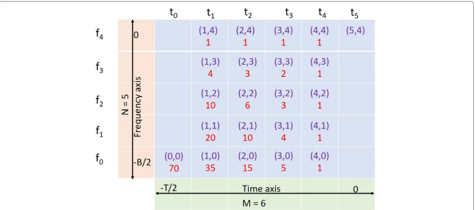
We will demonstrate this process of computing the
number of frequency paths K(m,n) going through
(tm,f(tm))with an example whereM = 6 and N = 5. The final results of this example are shown in Fig. 6. Due to the antisymmetric nature of the frequency func-tion, it is enough to generate only the first half of the frequency function. Each cell shows the values of(m,n) above the valueK(m,n). Hence, for this example, the fre-quency starts at−B/2 at time−T/2 denoted by location
(t0,f0)and ends at frequency 0 at time 0 denoted by
loca-tion(t5,f4). To compute the number of frequency paths
through each(tm,fn)locations, we start from the destina-tion(t5,f4). As given in step 1, the number of paths from
timet4isK(4,n)=1 forn=0, 1, 2, 3, 4, which we denote
in red font in locations(t4,f0)to(t4,f4)in the fourth
col-umn of the Fig.6. The number of frequency paths from the time pointst3tot0are computed as in step 2. For
exam-ple, the number of frequency paths through(t3,f3)is two
to one is(t3,f3) →(t4,f3) →(t5,f4), second is(t3,f3) → (t4,f4)→(t5,f4). We compute this number from step 2 as
K(3, 3) =K(4, 3)+K(4, 4)= 2. By following this proce-dure, we can compute the number of possible frequency paths for all (tm,fn) to (t5,f4) is the sum of frequency
paths from(tm+1,fn),(tm+1,fn+1) . . . (tm+1,f4). At timet0,
the only possible frequency location is f0, since it is the
Fig. 6All possible monotonically increasing frequency functions with six discrete time values and five discrete frequency values. Number of possible frequency paths for the given (time, frequency) combination is given by the number written below in red font. All frequency paths start at (0,0) and ends at (5,4)
of frequency paths from(t0,f0)to(t4,f5), we add all the
frequency paths from(t1,f1),(t1,f2),(t1,f3), and(t1,f4)as
K(0, 0)=
4
n=0
K(1,n)=35+20+10+4+1=70, (15)
which is shown in lower left location in Fig.6.
Once we have created the number of frequency paths table, the next step is to generate a frequency function. The frequency function starts from location (t0,f0). At
this location, there are 70 possible frequency functions. Thity-five of those frequency functions go through loca-tion(t1,f0), 20 of them go through(t1,f1), 10 of them go
through(t1,f2), four of them go through(t1,f3), and one of
them goes through(t1,f4). To randomly pick a frequency
path with uniform probability distribution, we choose a
random integer η from 1 to 70 inclusive with uniform
distribution. η will determine the choice of frequency
location at timet1as given below:
f(t1)=
⎧ ⎪ ⎪ ⎪ ⎪ ⎨ ⎪ ⎪ ⎪ ⎪ ⎩
f0, if 1≤η≤35
f1, if 36≤η≤55
f2, if 56≤η≤65
f3, if 66≤η≤69
f4, ifη=70.
(16)
From the selected frequency location at time t1, we
repeat this procedure for randomly selecting a frequency value att2. For example, say the frequency location att1is
f2. From this location, 10 frequency paths are possible as
shown in the Fig.6. Now we choose a random integerη
from 1 to 10 inclusive and the frequency location at time t2is
f(t2)=
⎧ ⎨ ⎩
f2, if 1≤η≤6
f3, if 7≤η≤9
f4, ifη=10.
(17)
Note in this case, the frequency values f0 and f1 are
not considered att2due to the monotonically increasing
characteristic of the frequency function. We repeat this procedure by selectingηwith uniform probability distri-bution for the remaining time instances till the frequency function reaches the destination (t5,f4) to get the first
half of the frequency function. We obtain the complete frequency function as
f(m)=
f(m), if 1≤m≤(M+1)/2
−f(M+1−m), if(M+1)/2+1≤m≤M. (18)
for oddMand
f(m)=
f(m), if 1≤m≤M/2
−f(M+1−m), ifM/2+1≤m≤M. (19)
for evenM.
Using this frequency function, we obtain the associated FM signal as
s(m) = exp
2πj m
l=1
f(l)t
. (20)
sin the signal set0only if it satisfies the AC mainlobe
width and bandwidth conditions mentioned in (1.1).
4.3 Experiment parameters and results
Using the procedure from Subsection 4.2, we generated
L=106random signals from the signal set0with
band-width B = 1000, time width T = 0.1, and number of
samplesM = 1001. We find the best randomly picked
signal with respect to the cost metricQ(s;β)for different
weightsβ. The magenta curve (solid line with diamond
shaped markers) in Fig.5corresponds to the cost of the best random signals selected for each weightβ. We can observe that the performance of the best random signals are in the same range as most of the parameterized sig-nal sets. But none of these random sigsig-nals outperform the best low dimensional signal sets for all the consid-ered weights (6D-OPFS signal forβ = 0, 0.25, 0.50, 0.75
and Price’s signal for β = 1.00). Hence, as we argued
in the beginning of this section, with 95% of confidence level, we estimate that 6D-OPFS and Price’s signal outper-form a fraction of at least(1− 1036) = 99.9997% of the
random signals from the signal set0. From the
simula-tion, we can infer that searching for the best radar signal from the 6D-OPFS and Price’s signal models require much less computational resources with small degradation in performance.
5 Conclusion
In this paper, we searched for the best FM signal with primary objective of minimizing AC sidelobes that are characterized by PSLR and ISLR. Apart from the AC side-lobe levels, the signal has to satisfy other constraints such as AC mainlobe width and IBER. The frequency func-tions of the FM signals proposed in the literature have monotonically increasing frequency functions with anti-symmetry around the temporal midpoint. We referred to the set of signals with such frequency function and also satisfying the AC mainlobe width and IBER con-straints as0. Many researchers have proposed
parame-terized FM signals that are in subsets of0. We searched
for the best FM signal from these parameterized sig-nal subsets of 0. To find the best signal, we defined
cost functions that are convex combinations of PSLR and ISLR with the objective of penalizing the AC sidelobes. We found that the 6D-OPFS signal model proposed in this paper outperforms other signal models for most of the convex combinations and Price’s signal model
out-performs other signal models for β = 1. But the best
radar signal may be from the random signal element of
the signal set 0 and not from the parameterized
sig-nal subsets. It is informative to find the proportion of the random signal elements that 6D-OPFS and Price’s sig-nal outperforms with certain confidence interval. From the argument we presented in Section4, we expect with
95% confidence that 6D-OPFS and Price’s signals outper-form at least 99.9997% of the randomly picked signals from0.
Appendix
Cook’s NLFM Using SPP:C
Cook [1] designed NLFM signals whose PSDs have a shape of cosn(f). In his paper Cook presented the group delays as a function of frequency for n = 1, 2, 3, 4. Withτn(f) denoting the group delay for a given value ofn, we have
τ1(f)=
The frequency functionf(t)is given by the inverse func-tion of group delayτn(f),τn−1(t):
f(t)=τn−1(t). (25)
Price’s NLFM:D
Price’s NLFM [2] has a two dimensional parameterD = [BLBC] to control the nonlinearity of the frequency func-tion,
These parameters also control the signal bandwidth. We modify this frequency expression slightly to
f(t,Bl,Bc)=B the parameter search space independent of the signal bandwidth. This change also reduces the parameter space which will facilitate the optimization routines to converge on more appropriate parameter set.
Collins and Atkins NLFM:E
In [5], Collins and Atkins proposed a NLFM frequency
con-trol the nonlinearity and suggested that parameter values around [ 0.5, 1.4] minimizes the peak sidelobe level.
f(t,α,γ )= B
They also proposed an amplitude weighting function to reduce the sidelobe level. It is possible to find amplitude weighting functions for the other NLFM signal models also to reduce the sidelobes. That activity is beyond the scope of this paper and we will limit the signals to have constant envelope so that we can have fair comparison with the other signal models.
Wenzhen–Yan:F
Wenzhen and Yan [7] designed a NLFM frequency
func-tion with the intenfunc-tion of achieving a PSD whose shape resembles a Blackman window [26]. Such a PSD will result in small AC sidelobes. Their frequency function
f(t,k1,k2) = Bk1tan(k2t/T) (29)
has two parameters F =[k1 k2]. Wenzhen and Yan
suggested the parameter values around [0.1171 2.607] to minimize AC sidelobes.
Vizitiu NLFMs:GandH
In [13], Vizitiu proposed two NLFM frequency functions that belong to the family of distorted LFM signal models.
The first frequency function has two parametersG =
[δfδt] in an arcsin based distortion function and is shown in (30) below. The second frequency function has three parameters H =[n δf δt] and a tn based distortion function and is shown below in (31).
f(t,δf,δt)=
AC: Auto correlation; AF: Ambiguity function; ATEFM: Antisymmetric time exponentiated frequency modulation; FM: Frequency modulation; IBER: In-band energy ratio; ISLR: Integrated sidelobe ratio; LFM: Linear frequency modulation; MF: Matched filter; MLW: Main lobe width; NLFM: Nonlinear frequency modulation; OPFS: Odd polynomial frequency signal; PSD: Power spectral density; PSLR: Peak-to-sidelobe ratio; SPP: Stationary phase principle
Acknowledgements
Not applicable
Authors’ contributions
Both authors contributed equally to the conception of the paper. SA was responsible in creating the simulation results and drafting the paper. GAW was responsible in interpreting the simulation results and substantially revised the draft.
Funding
Not applicable.
Availability of data and materials
Not applicable.
Competing interests
The authors declare that they have no conflict of interest.
Received: 22 July 2019 Accepted: 4 December 2019
References
1. C. E. Cook, A class of nonlinear fm pulse compression signals. Proc. IEEE.
52, 1369–71 (1964).https://doi.org/10.1109/PROC.1964.3393 2. R. Price, inProc. of URSI National Radio Science Meeting. Chebyshev low
pulse compression sidelobes via a nonlinear fm, (Seattle, 1979) 3. N. Levanon, E. Mozeson,Radar Signals. (Wiley-IEEE Press, 2004).http://
books.google.com/books?id=l_2lHI9fVHUC. Accessed 13 Dec 2019 4. H. Meikle,Modern Radar Systems - Second edition. (Artech House
Publishers, Norwood, 2008)
5. T. Collins, P. Atkins, Nonlinear frequency modulation chirps for active sonar. IEE Proc. Radar Sonar Navig.146, 312–316 (1999).https://doi.org/ 10.1049/ip-rsn:19990754
6. C. Le´snik, Nonlinear frequency modulated signal design. Acta Phys. Pol. A.
116, 351–354 (2009)
7. Y. Wenzhen, Z. Yan, inProceedings of 2014 IEEE International Conference on Signal Processing, Communications and Computing (ICSPCC). A novel nonlinear frequency modulation waveform design aimed at side-lobe reduction, (2014), pp. 613–618.https://doi.org/10.1109/ICSPCC.2014. 6986266
8. P. Yichun, P. Shirui, Y. Kefeng, D. Wenfeng, inProc. IEEE Radar Conf. Optimization design of nlfm signal and its pulse compression simulation, (2005), pp. 383–386.https://doi.org/10.1109/RADAR.2005.1435855 9. J. M. Kurdzo, B. L. Cheong, R. D. Palmer, G. Zhang, inProceedings of 2014
International Radar Conference. Optimized nlfm pulse compression waveforms for high-sensitivity radar observations, (2014), pp. 1–6.https:// doi.org/10.1109/RADAR.2014.7060249
10. C. E. Cook, J. Paolillo, A pulse compression predistortion function for efficient sidelobe reduction in a high-power radar. Proc. IEEE.52(4), 377–389 (1964).https://doi.org/10.1109/PROC.1964.2927 11. H. D. Griffiths, L. Vinagre, Design of low-sidelobe pulse compression
waveforms. Electron. Lett,.30(12), 1004–1005 (1994).https://doi.org/10. 1049/el:19940644
12. E. D. Witte, H. D. Griffiths, Improved ultra-low range sidelobe pulse compression waveform design. Electron. Lett.40(22), 1448–1450 (2004). https://doi.org/10.1049/el:20046548
13. I. C. Vizitiu, Some aspects of sidelobe reduction in pulse compression radars using nlfm signal processing. Progress. Electromagn. Res. C.47, 119–129 (2014)
14. L. K. Patton, C. A. Bryant, B. Himed, inProc. IEEE Radar Conf. Radar-centric design of waveforms with disjoint spectral support, (2012), pp. 269–274. https://doi.org/10.1109/RADAR.2012.6212149
15. G. Lellouch, A. K. Mishra, M. Inggs, Design of ofdm radar pulses using genetic algorithm based techniques. IEEE Trans. Aerosp. Electron. Syst.
52(4), 1953–1966 (2016).https://doi.org/10.1109/TAES.2016.140671 16. S. W. Frost, B. Rigling, inProceedings of 2012 IEEE Radar Conference.
Sidelobe predictions for spectrally-disjoint radar waveforms, (2012), pp. 0247–0252.https://doi.org/10.1109/RADAR.2012.6212145 17. L. K. Patton, C. A. Bryant, B. Himed, in2012 IEEE Radar Conference.
Radar-centric design of waveforms with disjoint spectral support, (2012), pp. 0269–0274.https://doi.org/10.1109/RADAR.2012.6212149 18. H. He, P. Stoica, J. Li, in2010 2nd International Workshop on Cognitive
constraints for cognitive radar, (2010), pp. 344–349.https://doi.org/10. 1109/CIP.2010.5604089
19. S. Alphonse, G. A. Williamson, in2014 22nd European Signal Processing Conference (EUSIPCO). Novel radar signal models using nonlinear frequency modulation (Lisbon, 2014), pp. 1024–1028.http://ieeexplore. ieee.org/stamp/stamp.jsp?tp=&arnumber=6952344&isnumber=6951911 20. A. Aubry, V. Carotenuto, A. D. Maio, A. Farina, L. Pallotta, Optimization
theory-based radar waveform design for spectrally dense environments. IEEE Aerosp. Electron. Syst. Mag.31(12), 14–25 (2016).https://doi.org/10. 1109/MAES.2016.150216
21. H. D. Griffiths, L. Cohen, S. Watts, E. Mokole, C. J. Baker, M. Wicks, S. D. Blunt, Radar spectrum engineering and management: Technical and regulatory issues. Proc. IEEE.103, 85–102 (2015)
22. S. Boukeffa, Y. Jiang, T. Jiang, inProceedings of the IEEE 7th International Colloquium on Signal Processing and Its Applications. Sidelobe reduction with nonlinear frequency modulated waveforms, (2011), pp. 399–403. https://doi.org/10.1109/CSPA.2011.5759910
23. S. Alphonse, G. A. Williamson, inProceedings of IEEE Radar Conference (RadarCon). Estimation of radar signals using passive sensor network, (2015), pp. 1525–1530.https://doi.org/10.1109/RADAR.2015.7131238 24. MATLAB - Version 2017a, Global Optimization Toolbox - Version 3.4.2
(MathWorks, Natick, 2017)
25. F. Tuyl, R. Gerlach, K. Mengersen, The rule of three, its variants and extensions. Int. Stat. Rev.77(2), 266–275 (2009).https://doi.org/10.1111/j. 1751-5823.2009.00078.x
26. F. J. Harris, On the use of windows for harmonic analysis with the discrete fourier transform. Proc. IEEE.66(1), 51–83 (1978).https://doi.org/10.1109/ PROC.1978.10837
Publisher’s Note