Surface Approximation Using the 2D FFENN
Architecture
S. Panagopoulos
Institute for Communications & Signal Processing, University of Strathclyde, Royal College Building, Glasgow G1 1XW, UK
Email:[email protected]
J. J. Soraghan
Institute for Communications & Signal Processing, University of Strathclyde, Royal College Building, Glasgow G1 1XW, UK
Email:[email protected]
Received 27 August 2003; Revised 10 March 2004; Recommended for Publication by Bernard Mulgrew
A new two-dimensional feed-forward functionally expanded neural network (2D FFENN) used to produce surface models in two dimensions is presented. New nonlinear multilevel surface basis functions are proposed for the network’s functional expansion. A network optimization technique based on an iterative function selection strategy is also described. Comparative simulation results for surface mappings generated by the 2D FFENN, multilevel 2D FFENN, multilayered perceptron (MLP), and radial basis function (RBF) architectures are presented.
Keywords and phrases:neural networks, sea clutter, surface modeling.
1. INTRODUCTION
One of the main properties of feed-forward neural networks is that of learning an input-output mapping from a set of ex-amples characterizing a real system. The network is trained with some examples comprising an input signal and the de-sired response. The network weights are then modified, us-ing an adaptive optimization technique to minimize the dif-ference between the desired response and actual response. Two well-known feed-forward artificial neural networks are the multilayered perceptron (MLP) and radial basis
func-tion (RBF). Both networks have been termed as universal
approximators [1,2]. Their performance has been
demon-strated in various application areas such as linear and
nonlin-ear adaptive filtering [3], time series prediction [4], dynamic
reconstruction [5], and black-box modeling [6]. However,
these networks suffer from a number of drawbacks, such
as convergence characteristics and network topology selec-tion [7].
MLP networks traditionally employ sigmoidal activation functions that cannot model local nonlinearity optimally. Also, their nonlinear in-the-parameters structure requires complex and computationally intense learning algorithms, such as the backpropagation algorithm. Furthermore, there is no way to say whether a single hidden layer is optimum to support the MLP network learning or a way to specify the
exact number of hidden neurons required in order for a sys-tem to be generalizable.
On the other hand, RBF networks that traditionally em-ploy radial symmetric functions cover only small localized regions and therefore they cannot model global nonlinearity
well. Moreover, dealing with RBF networks’ great difficulty
is experienced in selecting the appropriate centers for the ra-dial basis functional expansion. Additionally, a large number of basis functions is usually required in order to cover high-dimensional input spaces. Nonetheless, simple learning algo-rithms may be used for training, as the RBF structure is linear in the parameters.
In this paper, the design of a new single hidden layer, lin-ear in the parameters, two-dimensional feed-forward func-tionally expanded neural network surface modeler (2D FFENN) is presented. Previously, a 1D FFENN has been
suc-cessfully applied to time series prediction [8,9] and
cochan-nel interference [10]. The aim of this new design is to explore
t1(k)
Input 1
t2(k)
Input 2
[1×N] Nonlinear functional expansion Function selector · · · WeightsWN
WN W3W2W1
Network outputy(k) −
Errore(k)
Desired outputsd(k)
MSLE
MSE
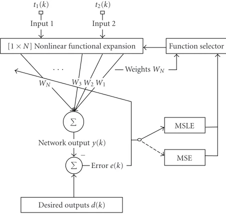
Figure1: The 2D FFENN structure.
The remainder of the paper is organized as follows. In
Section 2, an overview of the 2D FFENN and multilevel
2D FFENN architectures is given.Section 3provides a brief
description of the network weight adaptation algorithm.
Section 4 describes the characteristics of a function prun-ing technique, which is developed to optimize the network’s
functional expansion. InSection 5, a number of
representa-tive simulation results are presented that illustrate the surface modeling capabilities of both the 2D FFENN and multilevel 2D FFENN designs in comparison with the MLP and RBF
networks.Section 6concludes the paper.
2. THE 2D FFENN ARCHITECTURE 2.1. The 2D FFENN structure
The architecture of the 2D FFENN structure is depicted in
Figure 1. It consists of two layers: a single hidden layer and an output layer. The hidden layer acts like a feature detection layer. As the learning process progresses, the hidden neurons begin to gradually discover the salient features that charac-terize the training data. This is achieved by the functional ex-pansion unit, which performs a nonlinear transformation of the input data into a new space called the feature space. The output layer of the network comprises a set of linear combin-ers that join together all the weighted functionally expanded inputs to form a single output.
The functional expansion unit of 2D FFENN takes two
inputst1andt2which are the grid indices that specify the 2D
data set to be modeled. Both inputs are normalized to within
the range (+1,−1).
The entire functional expansion is described byF(k) as
follows:
F(k)=sum ofN(linear & nonlinear) basis functions.
(1)
In a similar fashion to the functions described in [11], the
linear terms of the expansion are the original input terms,
whilst the nonlinear terms are a combination of
trigonomet-ricandpolynomial2D functions of the input. The modeling
efficiency of the 2D FFENN is the result of this hybrid
func-tional expansion [12]. These functions have been chosen in
such a way to combine the global approximation capability of the MLP network’ the local approximation capability of the RBF network and also to emulate the modeling capability of the VNN.
In general, a multiple-input multiple-output (MIMO)
FFENN (n,N,m) will completely be specified for a given
number ofninputs andmoutputs by a similarF(k)
expan-sion.
The output of the two-layered, two-input, andN-term
FFENN (2,N, 1) is defined as follows.
(a) Hidden layer functional expansion vector at timek:
F(k)=f1(k),f2(k),. . .,fN(k) T
(2)
and the associated weight vector as
W(k)=w1(k),w2(k),. . .,wN(k) T
. (3)
(b) Single 2D FFENN output:
y(k)=FT(k)·W(k). (4) (c) Prediction error:
e(k)=d(k)−y(k), (5)
whered(k) is the reference response.
Network weight adaptation is achieved using the expo-nentially recursive least squares (RLS) algorithm. Complex training algorithms are not required because of the linear in-the-parameters network structure.
The function selection unit shown inFigure 1is used in
order to reduce the size of the functionally expanded net-work. The scope of the functional expander is to introduce to the network new functional terms in order to enhance its nonlinear approximation ability. However, this process can lead the expansion to very large and highly redundant networks. For this reason, a pruning or function selection scheme is occupied to choose only the most significant func-tions.
2D FFENN functional expansion
Analytically, the functional expansion of 2D FFENN, for 2
inputs (x1andx2) normalized within the range (+1,−1), is
described by the following set of terms.
(1) Zero-order (dc) term (1 term).
(2) Original input terms (2 terms). Linear system model-ing.
(3) Sine expansion of the 2 inputs, comprising sin(xi),
sin(2xi), and sin(3xi) terms fori=1, 2 (6 terms).
(4) Cosine expansion of the 2 inputs, comprising cos(xi),
(5) Cross input and sine expansion of the 2 inputs, com-prisingxisin(xj),xisin(2xj), andxisin(3xj) terms for
i=j,i,j=1, 2 (6 terms).
(6) Cross input and cosine expansion of the 2 inputs, com-prisingxicos(xj),xicos(2xj), andxicos(3xj) terms for
i=j,i,j=1, 2 (6 terms).
(7) Cross sine expansion of the 2 inputs, compris-ing sin(xi) sin(xj), sin(xi) sin(2xj), and sin(xi) sin(3xj) terms fori=j,i,j=1, 2 (5 terms).
(8) Cross cosine expansion of the 2 inputs, comprising cos(xi) cos(xj), cos(xi) cos(2xj), and cos(xi) cos(3xj) terms fori=j,i,j=1, 2 (5 terms).
(9) Cross cosine and sine expansion of the 2 inputs, comprising the terms cos(xi) sin(xj), cos(xi) sin(2xj), cos(xi) sin(3xj), cos(2xi) sin(xj), cos(3xi) sin(xj), cos(2xi) sin(3xj), cos(3xi) sin(2xj), cos(2xi) sin(2xj), and cos(3xi) sin(3xj) fori= j,i,j=1, 2 (18 terms). (10) Cross input and cosine and sine expansion of the 2
in-puts, comprisingxkcos(xi) sin(xj),xkcos(xi) sin(2xj),
The set of equations described above comprise the full cross-terms functional expansion. However, a number of these can be discarded due to the symmetric properties of the functions. The following functions may be excluded after visual inspection of the surface characteristics of all 80 function terms: sin(x2) sin(2x1), cos(x2) cos(2x1), The final functional expansion has been reduced to 59 functions in total.
2.2. Multilevel 2D FFENN design
The multilevel 2D FFENN design is an extended version of the generic 2D FFENN model. It incorporates extra
func-tion groups at different scales in order to enhance its
perfor-mance and to cope with “spikier” data. The topology of the
multilevel 2D FFENN design is depicted inFigure 2. The 2D
FFENN scale-set-1 unit (low-scales functional expansion)
shown inFigure 2refers to exactly the same design described
so far by the generic 2D FFENN using 59 functions. Scale-set-2 (medium-scales functional expansion) and scale-set-3 (high-scales functional expansion) are two additional func-tion groups that have been included in order to be intro-duced to the model functions at different scales. The network can produce results by either using scale-set-1 only, by using scale-sets-1 and -2, or by using all three sets together. Scale-set-2 achieves a further functional expansion of 33 functions and scale-set-3 adds an extra 42 functions at a higher scale.
Original
Figure2: The multilevel 2D FFENN design.
Extended 2D FFENN functional expansion
The extended functional expansion of the multilevel 2D FFENN is constituted by the following terms.
Medium-scales functional expansion
(1) Sine expansion of the 2 inputs, comprising sin(10xi)
and sin(20xi) terms fori=1, 2 (4 terms).
(2) Cosine expansion of the 2 inputs, comprising
cos(10xi) and cos(20xi) terms fori=1, 2 (4 terms).
(3) Cross sine expansion of the 2 inputs, comprising sin(xi) sin(10xj), sin(xi) sin(20xj), sin(10xi) sin(10xj), sin(20xi) sin(20xj), and sin(10xi) sin(20xj) terms for
i=j,i,j=1, 2 (8 terms).
(4) Cross cosine expansion of the 2 inputs, compris-ing the terms cos(xi) cos(10xj), cos(xi) cos(20xj),
cos(10xi) cos(10xj), cos(20xi) cos(20xj) and
cos(10xi) cos(20xj) fori= j,i,j=1, 2 (8 terms). (5) Cross cosine and sine expansion of the 2 inputs,
comprising cos(10xi) sin(10xj), cos(10xi) sin(20xj), cos(20xi) sin(10xj), and cos(20xi) sin(20xj) terms for
i=j,i,j=1, 2 (8 terms).
(6) Exponential expansion of the 2 inputs, comprising the following term:ecos(2·xi)+cos(2·xj), fori=j,i,j=1, 2 (1 term).
High-scales functional expansion
(1) Sine expansion of the 2 inputs, comprising sin(30xi)
and sin(40xi) terms fori=1, 2 (4 terms).
(2) Cosine expansion of the 2 inputs, comprising
cos(30xi) and cos(40xi) terms fori=1, 2 (4 terms).
(3) Cross sine expansion of the 2 inputs, comprising sin(xi) sin(30xj), sin(xi) sin(40xj), sin(30xi) sin(30xj), sin(40xi) sin(40xj), and sin(30xi) sin(40xj) terms for
i=j,i,j=1, 2 (8 terms).
(4) Cross cosine expansion of the 2 inputs, compris-ing the terms cos(xi) cos(30xj), cos(xi) cos(40xj),
cos(30xi) cos(30xj), cos(40xi) cos(40xj), and
cos(30xi) cos(40xj) fori= j,i,j=1, 2 (8 terms). (5) Cross cosine and sine expansion of the 2 inputs,
comprising cos(30xi) sin(30xj), cos(30xi) sin(40xj), cos(40xi) sin(30xj), and cos(40xi) sin(40xj) terms for
(6) Sigmoid expansion of the 2 inputs,
compris-ing tanh(xi), tanh(10xi), tanh(30xi), tanh(50xi),
tanh(60xi), and tanh(100xi) terms for i = 1, 2 (12
terms).
3. NETWORK WEIGHT ADAPTATION
FFENN network weight adaptation is achieved recursively by
the exponentially weighted RLS algorithm [13, Chapter13,
pages 562–587].
The exponentially weighted RLS estimator can be derived by minimizing the following cost function with respect to the
weight coefficient vectorW(k):
where the ensemble averages have now been replaced by time
averages andλrepresents a weighting or forgetting factor
be-longing to (0, 1).
The computation is launched with known initial condi-tions and then progresses recursively using information con-tained in new data samples that used to update the old esti-mates. The use of the exponential weighting factor or
forget-ting factorλ, in general, is intended to ensure that the data in
the distant past are “forgotten,” in order to allow modeling of time-variant systems.
The optimum weight vector W(k), for which the cost
function E(k) attains its minimum value, is defined by the
set of “normal” equations
Wopt=R−1(k)·Φ(k), (7)
where the autocorrelation matrixR(k) is defined as
R(k)= k
t=1
λk−t·F(t)·FT(t) (8)
and the cross-correlation vectorΦ(k) as
Φ(k)=
The inverse ofR(k) can then be estimated recursively using
the matrix inversion lemma [13, Chapter13, pages 562–587]
as follows. LetP(k) = R−1(k) and assumeΦ(k) is positive
definite and therefore nonsingular:
P(k)= 1
Hence, the final recursive update for the FFENN weight
vectorW(k), for a single output, can be expressed as
W(k)=W(k−1) +P(k)·F(k)·e(k). (14)
The RLS algorithm has been preferred due to its faster con-vergence rates, even though it is computationally more com-plex. A simpler algorithm such as the least mean squares (LMS) or the normalized least mean squares (NLMS) can equally be used.
The LMS algorithm uses a simple equation to update the
weight vectorW(k) as follows:
W(k+ 1)=W(k) + 2·µ·e(k)·F(k), (15)
whereµis the step-size parameter. Notice that the larger the
value ofµ, the faster the convergence of the weight vector, but
the more susceptible to noise.
For the NLMS algorithm, we need also to introduce the
normalized step-size parameterα. Thus, the step-size
param-eterµof (15) is now defined as
µ= α
F(k)·F(k)T, 0< α≤1. (16)
4. PRUNING OF THE FULLY EXPANDED 2D FFENN A large functional expansion can achieve better prediction results. Nevertheless, depending on the type and level of complexity of the surface to be modeled, the network may assume too many free parameters. This is because a much smaller number of functions are probably needed to charac-terize the specific function or surface. For this reason, a prun-ing scheme is utilized. Its task is to select only those functions which have a significant contribution to the output of the network. In other words, we want to choose only the domi-nant weights of the functional expansion.
Pruning is performed by an iterative pruning-retraining approach. Initially, the fully expanded network structure is trained on the training data set, and the maximum surface level error (MSLE) value on the training set is computed. For other methods, compute the mean square error (MSE) in-stead, which is defined as follows:
MSE=1
0.9
minimize localized error responses. In mathematical terms, the MSLE is defined as follows:
MSLE=maxe(k)−mine(k). (18)
The insignificant functions in the expansion model are as-sociated with the smallest weights; these are successively pruned one by one starting with the least significant one. Af-ter each insignificant function is being pruned, the output of the network is computed. Moreover, the resulting MSLE is also computed at each pruning stage. The pruning process is stopped at the stage when a pruned network structure is found to be incapable of reducing the output MSLE or MSE on the training set to the desired level. The network structure can be retrained after each time pruning is applied, with the same train set, in order to determine the optimal weights for the remaining unpruned functions.
Furthermore, it is important to note that pruning is only an optimization strategy and can be omitted when there is no advantage to be gained. It effectively achieves to reduce the size of the functional expansion, but in the downside, requires offline training (supervised learning) and much longer computation time.
5. SIMULATION RESULTS
5.1. Application to computer generated 2D data
5.1.1. Function approximation by the 2D FFENN and multilevel FFENN
In this section, we present simulation results for both the 2D FFENN and multilevel 2D FFENN structures. In order to il-lustrate the modeling capability of the 2D FFENN structure
and the effectiveness of the pruning strategy, we produce a
model for the smooth continuous surface described by (19).
The choice of this function is based on its surface character-istics that resemble the nature of a swell wave. It has also been
used in [14, Chapter 5, page 75] for testing the performance
×10−3
Figure4: Error surface of 2D FFENN (no pruning, 59 functions, 5 epochs).
of feed-forward neural networks:
Tt1,t2 =0.1 +
1 + sin2·t1+ 3·t2 3.5 + sint1−t2 .
(19)
Figure 3displays the surface characteristics of this 2D func-tion. The training set is constructed from the function
T(t1,t2) by sampling the domain from−1.0 to +1.0 in two
dimensions at equally spaced grid points, at an interval of 0.1
for botht1andt2. The 21 spacing indices generated for each
one of the dimensions correspond to the network inputs. InFigure 4, the 2D FFENN modeling error is presented. Modeling was achieved by a functional expansion of 59 func-tions and batch training was performed for 5 times. Pruning has not been considered, so at this stage, all 59 functions con-tribute to the model. Based on the results, we can conclude that the 2D FFENN is able to produce very good surface map-pings even after being trained for a small number of epochs. In order to test the efficiency of the pruning strategy em-ployed by the 2D FFENN, we simulate for the same surface, but this time using the MSE and MSLE to choose the most appropriate functions for modeling. The results are shown
in Figures 5and6, respectively. From the results, it is
evi-dent that pruning can effectively reduce the dimensionality of the functional expansion. MSLE measure considers the worst possible error (peak-to-peak error) achieving a fairly flat error response, while the MSE measures the average error and consequently fails to minimize localized error responses. In this example, 29 functions have been discarded. The size of pruning achieved mainly depends on the specific characteris-tics of the surface to be predicted and the number of training epochs. The algorithm allows the user to retrain also after each time pruning is performed. This leads to a better weight adaptation achieving a smaller mapping error. However, the downside is that the number of candidate-pruned functions is reduced. In general, the minimum the network training performed, the maximum the pruning that can be achieved.
Obviously, this tradeoffis directly reflected to the modeling
×10−4
Figure5: Error surface of 2D FFENN (MSE pruning, 30 functions, 5 epochs).
Figure 6: Error surface of 2D FFENN (MSLE pruning, 30 func-tions, 5 epochs).
results produced by the multilevel 2D FFENN design. The network is initially trained for a functional expansion of 134 functions and after 5 epochs of training, pruning manages to reduce the functional expansion down to 60 significant func-tions.
5.1.2. Comparative study
In this section, we compare the results presented in
Section 5.1.1with the performance of the MLP and RBF
neu-ral networks [7]. In order to perform a quantitative relative
comparison, we try to achieve the best surface approxima-tion that both the RBF and MLP can produce under a real-istic network design of a strength similar to that of the 2D FFENN.
In Figure 8, the MLP network training error is given. From the results, it appears to be inferior to the 2D FFENN. It requires 500 epochs under supervised batch training and ap-proximately a network expansion of 15 hidden neurons (i.e., 46 weights in total) to produce good but not better results than the 2D FFENN.
×10−4
Figure7: Error surface of multilevel 2D FFENN (MSLE pruning, 60 functions, 5 epochs).
×10−3
Figure8: MSLE error surface of MLP (500 epochs, 15 hidden neu-rons).
On the other hand, the RBF network can level the per-formance of the 2D FFENN at the expense of a large hidden neurons expansion. The associated training error for an RBF network of 42 hidden neurons (i.e., 127 weights in total) is
shown inFigure 9.
5.1.3. System validation
In order to validate the performance of the 2D FFENN, mul-tilevel 2D FFENN, MLP, and RBF networks, a test data set was constructed using grid spacing of 0.03195, a value cho-sen to avoid replication of training set points, forcing the net-work to interpolate. MSLE pruning was performed as it has proven to be a more reliable measurement in comparison to
the MSE. All results are shown inTable 1.
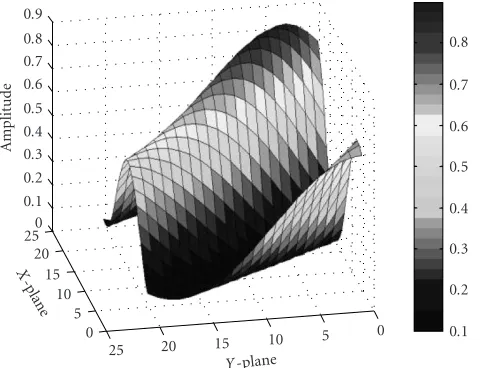
5.2. Application to real sea surface 5.2.1. Sea surface approximation
Table1: Network training and validation errors.
Network Pruning Total no. of weights Training MSLE Validation MSLE
2D FFENN Not applied 59 0.00259 0.00221
2D FFENN MSLE 30 0.00033 0.00030
Multilevel 2D FFENN MSLE 60 0.00029 0.00021
MLP Not applied 46 0.00785 0.00722
RBF Not applied 127 0.00104 0.00093
×10−4
6 4 2 0 −2 −4 −6
P
eak-t
o-p
eak
er
ro
r
1 0.5
0 −0.5
−1
Y-plane
−1 −0.6
−0.2 0.2
0.6 1
X-plane
Figure9: MSLE error surface of RBF (42 hidden neurons).
the performance of such systems. Sea clutter refers to the backscattered energy returns from a radar illuminated sea surface. A conventional radar system directs a beam of mi-crowave pulses illuminating a patch of the sea surface. The backscattered energy is collected and based on its strength and round trip delay targets can be detected and located. Sig-nal returns from the actual sea surface are widely known as sea clutter, whilst signal returns from an object are known as targets. Therefore, for successful target detection, sea clutter suppression must be achieved. Because sea clutter refers to radar signal returns from the sea surface itself, the problem casts explicitly to sea surface modeling.
In the previous section, we have demonstrated the mod-eling capability of the 2D FFENN design over two of the most well-known neural network architectures described in the lit-erature. In this section, we investigate the performance of the proposed 2D FFENN design to a real sea surface patch.
The actual sea surface texture segment is shown inFigure 10.
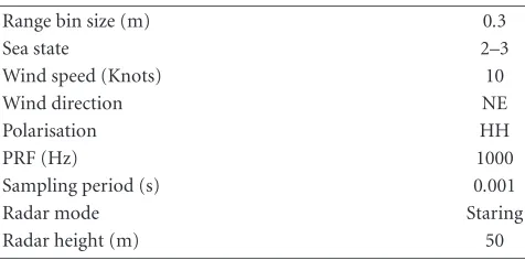
The data has been taken from a much larger radar data set, provided by QinetiQ, Malvern, with characteristics shown in
Table 2. Results have been produced for both the method of surface approximation by the 2D FFENN and MLP. The
cor-responding modeled surfaces are shown in Figures11and12,
respectively. The 2D FFENN network is initially trained for a functional expansion of 134 functions and after 10 epochs of training, pruning achieves reduction of the functional ex-pansion down to 97 significant functions (i.e., 97 weights in total). The MLP is trained for 500 epochs with a hid-den layer expansion of 32 neurons (i.e., 97 weights in total).
1.5 1 0.5 0
A
m
plitude
1 0.8 0.6 0.4 0.2 0−0.2−0.4−0.6−0.8 −1 Y-plane
1 0.6 0.2 −0.2 −0.6 −1
X
-plane
Figure10: Original sea surface.
Table2: Staring radar data (QinetiQ, Malvern, UK).
Range bin size (m) 0.3
Sea state 2–3
Wind speed (Knots) 10
Wind direction NE
Polarisation HH
PRF (Hz) 1000
Sampling period (s) 0.001
Radar mode Staring
Radar height (m) 50
From the surface approximation results, it is evident that both models are capable of estimating the main surface char-acteristics of the sea surface segment. Both models experi-ence some difficulty in estimating the sharp peaks of the ac-tual sea surface, however, the main peaks are clearly iden-tified. Modeling with the RBF network was not feasible, as the network was not able to approximate the original sur-face leading to a very large neuron expansion approaching the length of the original data.
6. CONCLUSION
1
Figure11: Error surface of multilevel 2D FFENN (MSLE pruning, 97 functions, 10 epochs).
1
Figure12: Error surface of MLP (500 epochs, 32 hidden neurons).
generated data and real sea clutter data were presented. A multiscaled functionally expanded structure of 2D FFENN design was also presented, designed to enhance its nonlinear modeling ability for surfaces where discontinuities and
spik-iness are present. An efficient function pruning strategy was
also devised. The results obtained by the proposed system demonstrate the effectiveness of such a network structure to produce surface mappings under short training times. Com-parative simulation results were also produced for MLP and RBF networks, validating the surface modeling potential of the 2D FFENN network architecture.
FFENN’s flexible functional expansion and short train-ing time makes it a very attractive design for many 2D sig-nal processing applications. We are currently extending the proposed network design to a wavelet-based functionally ex-panded structure. Our future development plans include first the extension of the static 2D FFENN architecture to a recur-rent 2D FFENN design, which will be able to produce
dy-namic models and second the extension of the 2D structure to a three-dimensional volume modeler, 3D FFENN, which lies on straightforward modifications of the existing system.
ACKNOWLEDGMENTS
The authors are very grateful to QinetiQ, Malvern, in partic-ular Professor I. Proudler and Dr. S. Lycett, for their valuable suggestions and for providing the real sea clutter data used inSection 5.2. This research was sponsored by QinetiQ un-der the United Kingdom Ministry of Defence Corporate Re-search Programme CISP.
REFERENCES
[1] D. R. Hush and B. G. Horne, “Progress in supervised neural networks: What’s new since lippmann,”IEEE Signal Processing Magazine, vol. 10, no. 1, pp. 8–39, 1993.
[2] J. Park and I. W. Sandberg, “Universal approximation using radial-basis-function networks,” Neural Computation, vol. 3, no. 2, pp. 246–257, 1991.
[3] D. Lowe and A. R. Webb, “Time series prediction by adaptive networks: a dynamical systems perspective,” IEE Proceedings Part F: Radar and Signal Processing, vol. 138, no. 1, pp. 17–24, 1991.
[4] S. Haykin and J. Principe, “Making sense of a complex world [chaotic events modeling],”IEEE Signal Processing Magazine, vol. 15, no. 3, pp. 66–81, 1998.
[5] S. Haykin, S. Puthusserypady, and P. Yee, “Dynamic re-construction of sea clutter using regularized RBF networks,” inProc. IEEE 32nd Asilomar Conference on Signals, Systems & Computers, vol. 1, pp. 19–23, Pacific Grove, Calif, USA, November 1998.
[6] S. Haykin and H. Leung, “Chaotic model of sea clutter using a neural network,” inAdvanced Algorithms and Architectures for Signal Processing IV, vol. 1152 ofProceedings of SPIE, pp. 18–21, San Diego, Calif, USA, 1989.
[7] S. Haykin, Neural Networks—A Comprehensive Foundation, pp. 208, 293 & 762, Prentice Hall, Upper Saddle River, NJ, USA, 2nd edition, 1999.
[8] A. Hussain, J. J. Soraghan, and T. S. Durrani, “A new hybrid neural network structure for non-linear time series model-ing,” Journal of Computational Intelligence in Finance, vol. 5, no. 1, pp. 16–26, 1997, Special issue on hybrid neural net-works for financial time series forecasting.
[9] A. Hussain, J. J. Soraghan, T. S. Durrani, and D. R. Campbell, “A new neural network structure for modeling non-linear dy-namical systems,” inProc. IEEE International Workshop on Image and Signal Processing, Advances in Computational Intel-ligence, B. G. Mertzios and P. Liatsis, Eds., pp. 119–122, Else-vier Science Publishers, Manchester, UK, November 1996. [10] A. Hussain, J. J. Soraghan, and T. S. Durrani, “A new
adap-tive functional-link neural-network-based DFE for overcom-ing co-channel interference,” IEEE Trans. Communications, vol. 45, no. 11, pp. 1358–1362, 1997.
[11] A. Hussain and J. J. Soraghan, “FENN methodology: Im-proved neural network,” UK Patent no. 9624298.7, November 1996.
[12] A. Hussain, Novel artificial neural-network architectures and algorithms for non-linear dynamical system modelling and dig-ital communications applications, Ph.D. thesis, Strathclyde University, Glasgow, UK, September 1996.
[14] T. Masters, Practical Neural Network Recipes in C++, Aca-demic Press, San Diego, Calif, USA, 1993.
[15] K. D. Ward, “Compound representation of high resolution sea clutter,” Electronics Letters, vol. 17, no. 16, pp. 561–563, 1981.
[16] H. Leung and S. Haykin, “Is there a radar clutter attractor?” Applied Physics Letters, vol. 56, no. 6, pp. 593–595, 1990. [17] J. L. Noga, Bayesian state-space modelling of spatio-temporal
non-Gaussian radar returns, Ph.D. thesis, Cambridge Univer-sity, Cambridge, UK, March 1999.
[18] M. Davies, “Looking for nonlinearities in sea clutter,” in IEE/EUREL Workshop on Radar and Sonar Signal Processing, Peebles, Scotland, July 1998.
[19] S. Haykin and S. Puthusserypady, Chaotic Dynamics of Sea Clutter, John Wiley & Sons, New York, NY, USA, 1999. [20] M. Cowper and B. Mulgrew, “Nonlinear processing of high
resolution radar sea clutter,” inProc. IEEE International Joint Conference on Neural Networks (IJCNN ’99), vol. 4, pp. 2633– 2638, Washington, DC, USA, July 1999.
S. Panagopoulos was born in Aegina, Greece, in 1977. He received the B.Eng. (honors) degree in electronic and electri-cal engineering from Strathclyde University, Glasgow, UK, in 2000. He is currently work-ing toward the Ph.D. degree in the Institute for Communications and Signal Processing, University of Strathclyde, Glasgow, UK. His current research interests include nonlinear time series modeling, wavelets, neural
net-work design, chaotic analysis, radar sea clutter suppression, and target detection.
J. J. Soraghanholds the Texas Instruments Chair in signal processing in the Institution of Communications and Signal Processing, Department of Electronic and Electrical En-gineering, University of Strathclyde, Glas-gow, Scotland. He received his B.Eng. de-gree with first-class honours in 1978 and his M.Eng.Sc. degree in 1982 both from University College Dublin, Ireland. He re-ceived his Ph.D. degree in electronic