R E S E A R C H
Open Access
Mean square error optimal weighting for
multitaper cepstrum estimation
Maria Hansson-Sandsten
Abstract
The aim of this paper is to find a multitaper-based spectrum estimator that is mean square error optimal for cepstrum coefficient estimation. The multitaper spectrum estimator consists of windowed periodograms which are weighted together, where the weights are optimized using the Taylor expansion of the log-spectrum variance and a novel approximation for the log-spectrum bias. A thorough discussion and evaluation are also made for different bias approximations for the log-spectrum of multitaper estimators. The optimized weights are applied together with the sinusoidal tapers as the multitaper estimator. Comparisons of the cepstrum mean square error are made of some known multitaper methods as well as with the parametric autoregressive estimator for simulated speech signals.
Keywords: Cepstrum; Log-spectrum; Multitaper; Mean square error; Optimal; Statistics; Bias; Variance
1 Introduction
Cepstrum-based methods are important in many applica-tions, especially speech analysis [1], and also in other areas such as, e.g., seismic deconvolution [2], vibratory diagno-sis using mechanical signals [3], and estimation of peri-ods of surface waves traveling around the circumference of tree trunks [4]. Usually, an autoregressive (AR)-based spectrum or a windowed periodogram is used for estima-tion of the cepstrum coefficients. The errors caused by bias and variance might be large, and algorithms based on robust spectrum analysis techniques could be useful for better performance. Such methods, usually derived from the periodogram, have been proposed lately, e.g., cepstrum coefficient thresholding in [5] and a novel tech-nique for power compensation of bias in [6]. In [7], a method for smoothing of the covariance function is pre-sented.
The concept of multiple windows or multitapers was invented by David Thomson [8,9], but multitapers were actually used much earlier in the form of one window shifted in time, the Welch method or Weighted Overlap Segmented Averaging (WOSA) by Welch [10]. The main idea of multitapers is to reduce the variance of the peri-odogram by averaging several uncorrelated periperi-odograms. The time-shifted window by Welch gives uncorrelated
Correspondence: [email protected]
Centre for Mathematical Sciences, Mathematical Statistics, Lund University, Box 118, Lund SE-221 00, Sweden
periodograms as the time-shifted window overlaps differ-ent data sequences, although the same window was used. The idea by Thomson was to use the same data sequence for all periodograms, i.e., the whole data sequence, but to change the shape of the window for the different peri-odograms in a way that gave uncorrelated periperi-odograms and thereby reduced variance. For smooth spectra, the Thomson multitaper method is used [8], but for spectra with larger dynamics and peaks, the peak matched multi-ple windows [11], the sinusoidal multitapers [12], and also more advanced multitaper methods, such as the adap-tive Thomson method [8], have been shown to be more suitable.
A preliminary mean square error optimal multitaper cepstrum estimator has been suggested in, e.g., [13] where the optimal multitapers and weights for a comb-spectrum model were used. This estimator has been evaluated and compared with the Thomson multitapers, the sinu-soidal multitapers, the Welch method, and usual win-dowed periodogram-based cepstrum analysis methods for speaker recognition. The results of these studies show that a multitaper estimator optimal for a speech-like spectrum model has advantages compared to traditional techniques [14-16].
The aim of this paper is to find a mean square error optimal weighting of the multitaper cepstrum estima-tor, based on the approximative mean square error for
the spectrum. The expression for the bias of the log-periodogram of a Gaussian process has been proposed and thoroughly evaluated in [6,17]. For the sinusoidal multitapers, the properties of the log-spectrum of locally white noise were derived in [18]. In [19], a more accurate expression for the bias was proposed. The attempt in this paper is to further simplify the expression of the bias of the log-spectrum using different Mercator series and to use such an approximation together with the Taylor expansion of the variance of the multitaper log-spectrum [18,19] to find mean square error optimal weights of the multitaper cepstrum.
The outline of the paper is as follows: In Section 2, suggestions of the approximative statistics for the cep-strum and log-spectrum are presented. Section 3 presents and evaluates mean square error optimal weighting fac-tors for the log-spectrum. In Section 4, evaluation and comparison of the mean square error of the cepstrum for speech-like processes are given. The paper is concluded in Section 5.
2 Approximative statistics of the multitaper log-spectrum estimate
From the discrete-time stationary stochastic processx(n), with spectral densitySx(f), the windowed periodogram is estimated as script T denotes the transposed vector. The multitaper spectrum is computed as
ˆ
using different window functionshk(n)in Equation 1 and weights,αk,k = 0. . .K −1. The window functions are normalized to give the expected valueE[Sˆk(f)]= Sx(f) forN→ ∞fork=0. . .K−1. The estimate of the real-valued symmetrical multitaper cepstrum is then defined as
for all integer values ofn, with log as the natural logarithm. The total mean square error (MSE) of the cepstrum esti-matorˆrc(n)and corresponding log-spectrum estimator is defined as tral density, respectively. The mean square error at the frequency valuef can be divided into
E logSˆx(f)−logSx(f)
whereV[∗] denotes variance.
2.1 Expected value and bias of the log-spectrum
A well-known expression for the expected value of the log-periodogram of a Gaussian process (see, e.g., [17]) is
E
whereγ ≈ 0.577 is the Euler constant. For the logarithm of a multitaper periodogram using the sinusoidal tapers, it was shown in [18] that the expected value is
ElogSˆx(f)
≈logESˆx(f)
+ψ (K)−log(K), (7)
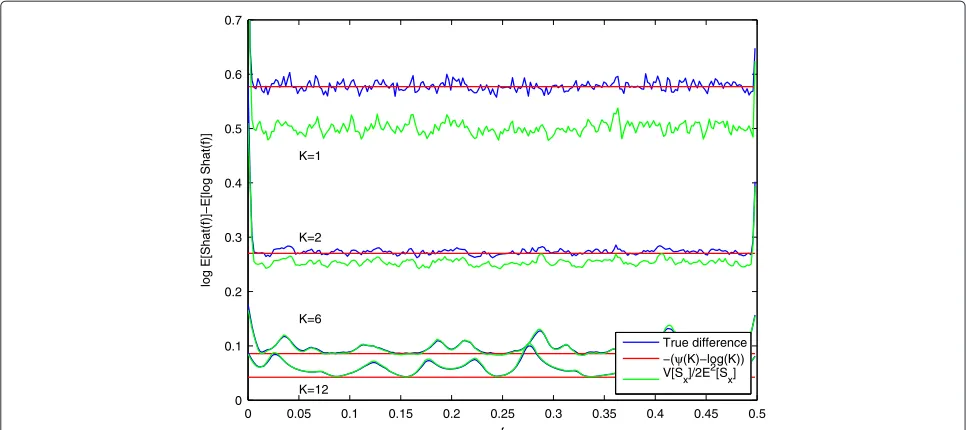
with equality for locally white noise. This equality is also expressed in [6] for the log-periodogram and also includes super-Gaussian and sub-Gaussian distributions of spec-tral coefficients. The number of multitapers is K, and ψ (K)is the digamma function, which can be recursively computed asψ (K+1) = ψ (K)+ K1 withψ (1) = −γ. For the case of K = 1, Equations 6 and 7 coincide, but for larger values ofK, the differenceψ (K)−log(K) approaches zero, e.g., forK=2,ψ (2)−log(2)≈ −0.270, and forK =6,ψ (6)−log(6)≈ −0.0856.
To verify if Equation 7 also holds for a varying spec-trum, a simulated example is shown in Figure 1 show-ing the difference (logESˆx(f)
0 0.05 0.1 0.15 0.2 0.25 0.3 0.35 0.4 0.45 0.5
and proposed approximations for different numbers of multitapers
K.
becomes larger over the different frequency values. How-ever, for varying spectrum and especially speech-like pro-cesses, a more accurate Taylor expansion approximation is defined by (green lines) is shown to be very similar to the true difference for higher value ofK(e.g.,K=6, 12).
Thetrue log-spectrum bias(TLSB) is
bias=ElogSˆx(f)
−logSx, (9)
and using the definition from Equation 7 and extending from locally white noise, the approximate log-spectrum bias(ALSB) is defined as
bias ≈ logESˆx(f)
An expansion of the term logE applied although often referred to as inaccurate. Replacing
1+x= E and the best approximation is given when E
ˆ
Sx
Sx is close
to 1, i.e., the expected value is close to the true spectrum. The two first terms in a more thorough approximation are used, referred to astwo-term true spectrum normalized bias approximation, TNBA(2),
bias≈
A simpler approximation is proposed for comparison, referred to as one-term true spectrum normalized bias approximation, TNBA(1), Equation 10 is also neglected, as this term, for the multi-taper case, is small compared to the error in the omitted higher-order terms.
Using a Euler expansion on the above Mercator series gives another Mercator series as log
logE[Sˆx(f)]
Similarly, as above, the bias approximation
bias≈
is referred to as thetwo-term expected value normalized bias approximation, ENBA(2). A simpler approximation, one-term expected value normalized bias approximation, ENBA(1),
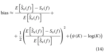
is also suggested. The ALSB, TNBA(2), and ENBA(2) will give about the same values for the single window case (K = 1), but for the multitaper log-spectrum, the dif-ferences might be substantial. This is illustrated with an example in Figure 2 where 10,000 realizations of the same AR(12) process as above are used. The number of win-dows isK=6 sinusoidal multitapers, and in Figure 2a, the
relative expected value of the spectrum, E
ˆ
Sx
Sx , is depicted to show that the relative value is quite close to 1, or at least between 0 and 2 for the whole spectrum, which indicates that the approximation referred to as TNBA would be appropriate. In Figure 2b,c, the error between the different bias approximations compared to the true bias of the log-spectrum in Equation 9 is shown. Note that the error for the ALSB (blue line) is the same in both Figure 2b,c. For this highly varying spectrum, we see that the ALSB is a fair approximation and that TNBA(2) as well as the TNBA(1) gives very large errors for the cases
where E f = 0.40. The ENBA(2) gives in these cases a smaller error (see Figure 2b) but might also give a much larger error than the TNBA(2). The more simple approximation of TNBA(1) and ENBA(1) in Figure 2c gives larger errors.
However, at the peaks of the spectrum, i.e.,f =0.05, 0.10, 0.20, 0.30, 0.35, and 0.40, the difference of the errors com-pared to Figure 2b is not that large, but at the smooth parts, between the peaks, the negative effect of omitting the termψ (K)−log(K)is notable. For larger values of K, this error will be smaller as this term also becomes smaller for largerK.
2.2 Variance of the log-spectrum
Expressions for the variance of the log-spectrum have been derived, e.g., the variance of the log-periodogram of a Gaussian process was derived in [17] and shown to be
V
This result was generalized in [6] to hold for complex super-Gaussian as well as sub-Gaussian spectral coeffi-cients. For the logarithm of multitaper spectra using K sinusoidal tapers, it was shown in [18] that the variance, with a locally white noise assumption, is
V
logSˆx(f)
=ψ(K), (17)
whereψ(K)is the trigamma function and is recursively computed byψ(K+1) = ψ(K)− K12 andψ(1) = π
2 6 (trigamma).
The approximation based on the Taylor expansion sug-gested in [7], i.e.,
was shown to be a sufficiently accurate approximation for speech-like processes. This approximation is referred to asexpected value normalized variance approximation (ENVA).
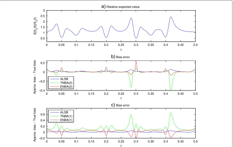
To compare these approximations, 10,000 realizations from the AR(12) process above are used. The results are presented in Figure 3 for different values ofK. The true variance of the log-spectrum is presented as the blue line, and forK = 1, this coincides very well withψ(1) = π62 (cyan). The ENVA, as the red line, is not at all close to the true variance. However, whenKincreases, the ENVA and the true variance coincide very well, also in the vari-ations of the spectrum, where the approximation from Equation 17 does not fit that well.
3 Mean square error optimal weighting of the multitaper cepstrum
0 0.05 0.1 0.15 0.2 0.25 0.3 0.35 0.4 0.45 0.5 0.5
1 1.5 2 2.5 3
f
E[S
x
(f)]/S
x
(f)
a)
0 0.05 0.1 0.15 0.2 0.25 0.3 0.35 0.4 0.45 0.5
−0.4 −0.2 0 0.2
f
Approx. bias − True bias
b)
0 0.05 0.1 0.15 0.2 0.25 0.3 0.35 0.4 0.45 0.5
−0.2 0 0.2 0.4 0.6
f
Approx. bias − True bias
c)
Relative expected value
Bias error
Bias error ALSB
TNBA(2) ENBA(2)
ALSB TNBA(1) ENBA(1)
Figure 2Example of relative expected value and the differences between approximative bias and true bias.(a)The relative expected value
EˆSx(f)
/Sx(f).(b)The difference between the approximative bias and the true bias of ALSB, TNBA(2), and ENBA(2).(c)The difference between the approximative bias and the true bias of ALSB, TNBA(1), and ENBA(1). A simulated AR(12) process is used with 10,000 realizations.
the mean square error for each frequency is chosen as
MSEf =
ElogSˆx(f)
−logSx(f)
2
+VlogSˆx(f)
,
(19)
≈
E[Sˆx(f)]−Sx(f)
E[Sˆx(f)]
2
bias2
+ V[Sˆx(f)]
E2[Sˆx(f)] variance
,
(20)
where ENBA(1) and ENVA are applied as approximations of the bias and variance of the log-spectrum, respectively. This approximation shows thatnormalizing the sum of all MSEf of the spectral estimatorSˆx(f)with the squared expected value of Sˆx(f) gives a reasonable approxima-tion of the mean square error for the estimator logSˆx(f) and is thereby also related to the MSE of Equation 4. It is therefore reasonable to assume that minimization of Equation 20 for allf, also minimizing Equation 4, would give an optimal estimator for the cepstrum coefficients ˆ
rc(n).
The bias in Equation 20 using the multitaper spectrum estimator of Equation 2 is
bias= K−1
k=0αkhTkH(f)Rx(f)hk−Sx(f)
K−1
k=0 αkhTkH(f)Rx(f)hk
, (21)
where Rx = E[xxT], (f) = diag[1 e−i2πf. . .
e−i2π(N−1)f] and the superscript H denotes conjugate transpose. The variance is
variance= K−1
l=0 K−1
k=0αlαkcov[Sˆk(f)Sˆl(f)]
(Kk=0−1αkhTkH(f)Rx(f)hk)2
, (22)
where cov[Sˆk(f)Sˆl(f)]= |hTkH(f)Rx(f)hl|2 + |hTk (f)Rx(f)hl|2. The second term is large only for fre-quencies close to f = 0 or to the Nyquist frequency, where the function hTk(f)Rx(f)hl overlaps its con-jugate. Most of the spectrum power is however located at the frequencies in between. The covariance for the frequencyf is therefore approximated as
0 0.1 0.2 0.3 0.4 0.5 0
0.5 1 1.5 2
f
Variance
K=1
True ENVA Trigamma
0 0.1 0.2 0.3 0.4 0.5
0 0.2 0.4 0.6 0.8 1
f
Variance
K=2
True ENVA Trigamma
0 0.1 0.2 0.3 0.4 0.5
0 0.1 0.2 0.3 0.4
f
Variance
K=6
True ENVA Trigamma
0 0.1 0.2 0.3 0.4 0.5
0 0.1 0.2 0.3 0.4
f
Variance
K=12
True ENVA Trigamma
Figure 3The true variance, ENVA, and the approximation from Equation 17 for different numbers of multitapersK.
The optimization criterion of Equation 20 includes the expressions of Equations 21 and 23 with unknown hk andαk,k = 0 . . . K− 1. In the further optimization, the multitapers hk are assumed to be known and to be the sinusoidal tapers of [12] with N = 256. The only unknowns are the weighting factorsαk,k=0 . . . K−1, which however appear both in the numerator and the denominator.
The choice of multitapers is crucial, and for an appli-cation where the data can be expected to originate from a highly dynamical spectrum, the Slepian multitapers [8] could be a better choice. The concern in this paper is based on the application to speech signals, where the spec-trum can be expected to have peaks, usually not too sharp, and in total a reasonable dynamics.
In all periodogram-based spectrum analysis methods, the multitaper estimation method can be considered to be a filtering procedure in a FIR-filter bank where the filter functions all can be modulated to be an identical base-band filter with center frequency 0. For each frequency, the input signal is consequently demodulated and filtered through the baseband filter [20]. As baseband filter, a sim-ple AR(1) spectrum is used, with a peak located at zero fre-quency, i.e., one pole inρ. The resulting optimal weights for two different cases ofρ are presented where the cor-responding covariance matrixRxis used in Equation 20. The AR(1) spectrum is a simple model but reasonable
for speech data as speech data often are estimated as AR models (order 10-20). The average damping of the differ-ent poles (ρ) of such an estimated AR spectrum from real data will give an idea of what damping factor should be chosen for the AR(1) model for the optimization of the weights. How this averaging and choice should be made is left for further studies.
The criterion is non-linear with respect to the unknown αk,k = 0 . . . K −1, and is therefore minimized itera-tively with a quasi-Newton algorithm [21]. This algorithm was presented in [22] and is also applied in this paper. The initial weighting factors are in all cases equal weights, αk=1/K,k=0 . . . K−1. In this paper, no further study of the convergence is made. The criterion MSEf can be optimized for different frequenciesf. Naturally, the peak frequencyf = 0 of the model spectrum is interesting, as well as the resolution, i.e., the bandwidth of the estimator [8,22]. The function to be minimized is
ξ=
W/2
fn=−W/2
MSEfn (24)
0 0.005 0.01 0.015 0.02 0.025 0.03 0.035 0.04 0.045 0.05 0
0.2 0.4 0.6 0.8 1
f
SAR
(f)
a) ρ=0.98 and bandwidths W.
W=0.02 W=0.04 W=0.08
0 5 10 15 20
0 0.1 0.2 0.3 0.4
k αk
b)
AR(1)−model spectra for
Optimal αk for the sinusoidal tapers.
OPT98 002 OPT98
004 OPT98
008
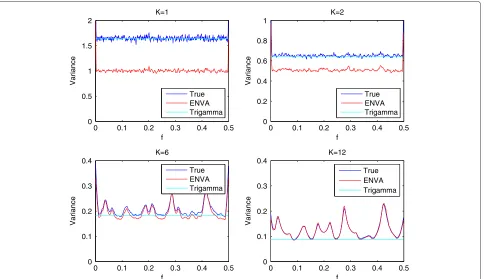
Figure 4Model spectrum forρ=0.98and optimal weighting factors.(a)The model spectrum AR(1) forρ=0.98 and the different optimization bandwidths.(b)Weighting factors from the optimization of the approximation of the mean square error of the log-spectrum, for the different bandwidths.
i = 0. . .N − 1, and the highest frequency taper to be included in the bandwidth|f| < W/2 is numberi =< W/2·2(N+1)giving K = i+1 < (W ·(N+1))+ 1. The chosen optimization bandwidth is crucial for the resolution of the final estimate, and it should be chosen
at least somewhat smaller than the preferred resolution of the final estimate as done in spectrum analysis. The local in-band multitaper cepstrum bias of the sinusoidal tapers is shown in [18] to be bounded by Sx(f)
Sx(f)
K2 24N2 for equal weights and can be expected to be smaller than for
0 0.005 0.01 0.015 0.02 0.025 0.03 0.035 0.04 0.045 0.05
0 0.2 0.4 0.6 0.8 1
f
SAR
(f)
a) ρ=0.93, and bandwidths W.
0 5 10 15 20
0 0.05 0.1 0.15 0.2
k αk
b)
AR(1)−model spectra for
Optimal αk for the sinusoidal tapers.
W=0.02 W=0.04 W=0.08
OPT93 002 OPT93
004 OPT93
008
Table 1 Evaluation ofξevof the optimal weighting OPT098 for different estimation and evaluation bandwidthsW
ξev(K) W=0.02 W=0.04 W=0.08
OPT098 0.563 (6) 0.424 (11) 0.301(21)
SINopt 0.618 (3) 0.532 (3) 0.423 (4)
THOMopt 0.674 (3) 0.572 (3) 0.453 (4)
WELCHopt 0.613 (4) 0.505 (4) 0.408 (4)
HAMM 1.91 (1) 1.92 (1) 1.93 (1)
ξevis the average log-spectrum MSE. The number of tapers giving the minimum errors for the sinusoidal tapers, Thomson multitapers and Welch method and the errors of the single Hamming window are also shown.
the Slepian multitapers. The Slepian multitapers, how-ever, have better leakage properties or out-of-band bias [8]. The sampling frequency of the actual process will effect an estimatedρas well as the decision of the band-width parameter W. For example, reducing the sample frequency by a factor of 2 will give half the number of data valuesN, which will increase the in-band bias by a fac-tor of 4, but the reduced number of samples will be fully compensated by the decrease ofρ. For the AR(1) model, the damping factor will change from ρ to ρ2, signifi-cantly affecting the spectrum shape to be more smooth. The bandwidth parameter W can be twice as large as the actual spectrum peaks of the data now which is a factor 2 further from each other compared to the non-reduced sampling frequency. The number of tapers will then be approximately the same as K ≈ W ·N, andN is reduced butW is doubled. Thereby, the variance will not change significantly. However, a reduction of sampling frequency is always beneficial, if possible, to the point where actual information is lost, but the further and more thorough analysis of the sampling effects is left for future research.
Three different bandwidths is used in the optimiza-tion, W = 0.02, 0.04, and 0.08, according to Figure 4a where the different vertical colored lines markW/2. The related number of tapers is K = 6, 11, and 21 for the respective bandwidth. The model spectrum is the AR(1) spectrum withρ = 0.98. The resulting weighting factors
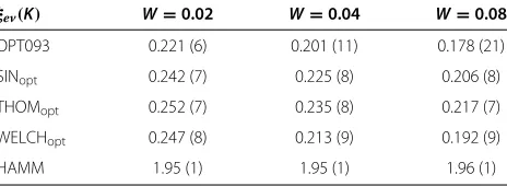
Table 2 Evaluation ofξevof the optimal weighting OPT093 for different estimation and evaluation bandwidthsW
ξev(K) W=0.02 W=0.04 W=0.08
OPT093 0.221 (6) 0.201 (11) 0.178 (21)
SINopt 0.242 (7) 0.225 (8) 0.206 (8)
THOMopt 0.252 (7) 0.235 (8) 0.217 (7)
WELCHopt 0.247 (8) 0.213 (9) 0.192 (9)
HAMM 1.95 (1) 1.95 (1) 1.96 (1)
ξevis the average log-spectrum MSE. The number of tapers giving the minimum errors for the sinusoidal tapers, Thomson multitapers and Welch method and the errors of the single Hamming window are also shown.
are depicted in Figure 4b where the blue line represents the K = 6,k = 0. . .5 values forW = 0.02, the green line the K = 11 values for W = 0.04, and the red line the resulting weighting factors for W = 0.08. The three curves are quite similar and are approaching zero for higherk, indicating that using the fewer weighting fac-tors from the narrow frequency bandW = 0.02 might work as well as the larger number from the optimization bandwidthW =0.08.
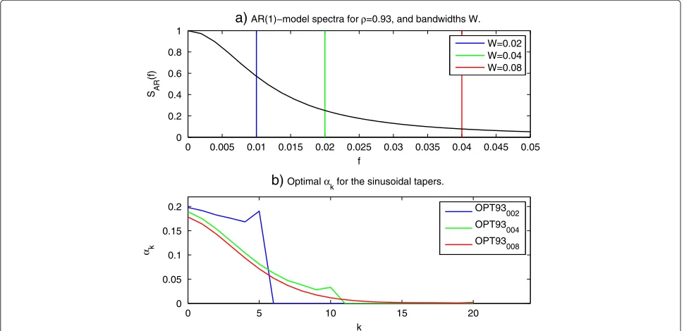
A more wideband process, the AR(1) process withρ = 0.93 (see Figure 5a), gives another result. Using the nar-row band for the optimization gives theK = 6 weighting factors depicted as the blue line in Figure 5b. These val-ues are quite close to each other, indicating that equally weighted mutitaper spectra might work as well for this type of spectrum. For a wider bandwidth, including more of the spectrum in the optimization, the resulting weight-ing factors are given by the green and red lines forW = 0.04 and 0.08, respectively.
To compare the actual performances of these approx-imative estimators, an evaluation of the mean square errors of the log-spectrum, i.e., Equation 19, is made for 10,000 realizations of an AR(2) process with the poles located at ρe±i2π0.25. The evaluation bandwidth is lim-ited to 0.25−W/2 ≤ f ≤ 0.25+W/2. The resulting mean square errors,ξev, using the proposed weighting fac-tors of Figures 4 and 5 and the sinusoidal tapers (N = 256), are calculated (OPT098 and OPT093). In Tables 1 and 2, the results are compared to the results of other well-known methods, such as (equally weighted) sinu-soidal tapers, the Thomson multitapers, and the Welch method (Hanning window and 50% of overlap), using the number of tapers that give the smallest error (SINopt, THOMopt, and WELCHopt). For comparison, the results using a single Hamming window are also computed (HAMM). For the more peaked spectrum (ρ = 0.98), the results for OPT098 are much better than for the equally weighted multitaper methods as well as the sin-gle Hamming window. The cost is the increased num-ber of tapers of the estimate. However, for OPT098 and W = 0.02, the number of tapers isK = 6, to be com-pared with K = 4 or K = 3 for the other multitaper methods. For the broadband spectrum with ρ = 0.93, the results of OPT093 are much better than the other multitaper methods even though, in the case of W = 0.02, the number of multitapers is actually fewer. These simulations are just a verification that the optimization has performed well, and the more interesting evaluation is for the total log-spectrum and thereby also for the cepstrum.
4 Cepstrum analysis of speech processes
Table 3 Cepstrumξcfor simulated AR processes, where the AR model is estimated from ‘A’ ofhallo
ξc(K,M) M1(49) M2(12) M3(14) F1(39) F2(12) F3(43)
OPT098002 0.546 (6) 0.323 (6) 0.323 (6) 0.583 (6) 0.322 (6) 0.554 (6)
OPT098004 0.532 (11) 0.294 (11) 0.290 (11) 0.582 (11) 0.290 (11) 0.531 (11)
OPT098008 0.529 (21) 0.259 (21) 0.257 (21) 0.590 (21) 0.245 (21) 0.522 (21)
OPT093002 0.703 (6) 0.208 (6) 0.223 (6) 0.734 (6) 0.202 (6) 0.746 (6)
OPT093004 0.693 (11) 0.176 (11) 0.194 (11) 0.724 (11) 0.158 (11) 0.689 (11)
OPT093008 0.673 (21) 0.182 (21) 0.191 (21) 0.716 (21) 0.156 (21) 0.663 (21)
SINopt 0.630 (3) 0.193 (8) 0.216 (7) 0.643 (4) 0.179 (8) 0.629 (3)
THOMopt 0.661 (3) 0.198 (8) 0.224 (7) 0.671 (3) 0.186 (8) 0.661 (3)
WELCHopt 0.590 (4) 0.186 (8) 0.205 (8) 0.633 (4) 0.167 (9) 0.608 (4)
HAMM 1.69 (1) 1.64 (1) 1.65 (1) 1.71 (1) 1.63 (1) 1.70 (1)
ARopt 0.964 (49) 0.165 (12) 0.140 (14) 0.362 (39) 0.281 (12) 0.611 (43)
There were six different speakers (three males and three females). The true model orders are noted for different speakers. The number of multiple windowsKis also given after the value ofξcfor the different methods. For the AR estimator, the estimated model orderMfor the minimum error is presented.
‘A’ of recorded data of the Swedish wordHallå(Hallo) as well as of the whole wordHallåfrom the same speakers (three males and three females). The reason for analyz-ing ‘A’ is the more stationary character of vowels duranalyz-ing the whole sequence length. However, the methods should also be robust against normal changes of the speech, and therefore the whole wordHallåis also investigated, where the sequences for the spectrum analysis are chosen sub-sequentially and without overlap. The total lengths of the differentHallåare between 248 and 567 ms, and the sam-pling frequency is 11 kHz, giving the number of sequences between 9 and 23 where the sequence length isN = 256 (23 ms). For the syllable ‘A’,N = 256 in all cases. The choice of the AR model order for each sequence is made from the Akaike information criterion (AIC). A number of 1,000 simulated speech-like processes are then produced
from the different models, and the evaluation criterion is the total mean square error for the cepstrum,
ξc= N−1
n=1
Erˆc(n)−rc(n)
2
. (25)
Note that the cepstrum coefficient atn= 0 is excluded in this analysis. The reason is that the zeroth coefficient corresponds to a constant energy level of the spectrum and is usually omitted in most cepstrum applications.
The estimators OPT098 and OPT093 from the for-mer section are applied and compared with THOMopt, WOSAopt, and SINoptas above where the result from the number of multitapers giving the smallest error is pre-sented. A comparison with an AR estimator is also made.
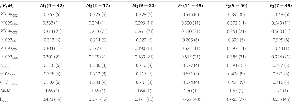
Table 4 Cepstrumξcfor simulated AR processes, where the AR model is estimated from different sequences ofhallo
ξc(K,M) M1(4−42) M2(2−17) M3(9−20) F1(11−49) F2(9−50) F3(7−49)
OPT098002 0.363 (6) 0.325 (6) 0.328 (6) 0.546 (6) 0.395 (6) 0.648 (6)
OPT098004 0.338 (11) 0.294 (11) 0.299 (11) 0.520 (11) 0.372 (11) 0.649 (11)
OPT098008 0.314 (21) 0.253 (21) 0.261 (21) 0.510 (21) 0.351 (21) 0.663 (21)
OPT093002 0.313 (6) 0.214 (6) 0.220 (6) 0.705 (6) 0.399 (6) 0.995 (6)
OPT093004 0.304 (11) 0.177 (11) 0.190 (11) 0.622 (11) 0.397 (11) 1.04 (11)
OPT093008 0.301 (21) 0.175 (21) 0.189 (21) 0.615 (21) 0.385 (21) 0.974 (21)
SINopt 0.316 (6) 0.200 (8) 0.210 (8) 0.627 (4) 0.3917 (5) 0.727 (3)
THOMopt 0.328 (6) 0.212 (8) 0.217 (7) 0.671 (3) 0.428 (5) 0.771 (3)
WELCHopt 0.302 (6) 0.203 (9) 0.201 (8) 0.624 (4) 0.422 (5) 0.716 (3)
HAMM 1.65 (1) 1.65 (1) 1.64 (1) 1.70 (1) 1.67 (1) 1.71 (1)
ARopt 0.428 (19) 0.361 (12) 0.171 (13) 0.722 (48) 0.663 (27) 0.635 (45)
The model order (using the AIC criterion) giving the smallest error is presented. The result of the single Ham-ming window periodogram (HAMM) is also added, as this method is often applied in speech analysis. The result of this method is however much worse than any of the multitaper methods.
In Table 3, the minimum total mean square errors ξc for the six different ‘A’ from three male and three female speakers are presented. For all subjects, the used simulation AR model orders are shown in the first line, e.g., order 49 was given for the first male speaker,M1(49). As expected, the order of the underlying model is found to be the optimal one in all cases for the AR estimator, ARopt. The estimated model orders are presented after the error of the ARoptin parenthesis. Similarly, the optimal num-ber of tapers for all the multitaper methods is expressed in parenthesis after the error.
Studying the errors of the multitaper methods, it can be seen that one of the proposed estimators, either OPT098 or OPT093 gives the smallest error in almost all cases followed by WELCHopt, SINopt, and THOMopt. In most cases, the number of tapers needed are just two or three more than for the equally weighted multitaper methods, e.g., forM1; the error given from OPT098002(K = 6) is much smaller than the error from WELCHopt(K = 4). Similarly, forF2, the error given from OPT093004(K=11) is substantially smaller than the error from WELCHopt (K = 9). In almost all cases, as expected from AR model simulations, the ARopt gives a much better result. How-ever, in several cases, the error of ARoptis much larger than the multitaper methods, e.g.,M1 andF2. It is also interesting to note that the error of the single Hamming window, HAMM, is almost the same for all speakers. This is in concordance with the expressions given in [6,17], where the bias is approximately zero and the total variance as well as the total mean square error isπ2/6≈ 1.64, for all cepstrum coefficients, excluding the zeroth coefficient. In Table 4, theaverageξcof subsequent intervals of the total wordHallåis presented (number of sequences differ between 9 and 23). For all cases, the same methods and the same parameter settings as in previous studies are evalu-ated. The ARoptis investigated for different model orders, and the model order giving the smallest total error for all subsequences ofHallåis used and the corresponding error is presented. The results of the multitaper meth-ods show about the same difference as for the evaluation the syllable ‘A’. At least one of OPT098 or OPT093 gives a smaller error than WELCHopt, SINopt, and THOMopt. Sometimes both OPT098 and OPT093 give a smaller error, e.g., forF1, which also is smaller than the error given by the ARopt, which is an indication of the robustness of the estimator against the choice of model. In most cases, a considerable reduction of the error is given from the OPT098 and OPT093 only using K = 6 or 11 tapers,
which is a reasonable additional number compared to the equally weighted multitaper methods (K = 3−9). The ARopt now shows a considerable larger error in several cases than the multitaper methods. Similarly as for the syl-lable ‘A’, the single Hamming window gives results around 1.64.
5 Conclusions
A cepstrum estimator is proposed based on a weighted multitaper spectrum. An evaluation of different approx-imations for bias and variance of the multitaper log-spectrum is made, and a mean square error criterion is proposed that includes novel approximations of the bias and variance. The weights of the multitaper spectrum are optimized, and the new estimator, the optimal weights combined with the sinusoidal tapers, is evaluated for cep-strum estimation of speech-like processes. The results show that a 10% to 20% reduction of the mean square error of the cepstrum can be achieved, to the cost of two or three additional periodogram computations.
Competing interests
The author declares that she has no competing interests.
Acknowledgments
The author would like to thank the Swedish Research Council for funding and also express gratitude to the anonymous reviewer that pointed out the similarity of the bias and variance formulas in [6] and [18].
Received: 22 April 2013 Accepted: 30 September 2013 Published: 17 October 2013
References
1. TF Quatieri,Discrete-Time Speech Signal Processing(Prentice Hall, Upper Saddle River, 2002)
2. JM Tribolet,Seismic Applications of Homomorphic Signal Processing
(Prentice Hall, Englewood Cliffs, 1979)
3. ME Badaoui, F Guillet, J Danière, New applications of the real cepstrum to gear signals, including definition of a robust fault indicator. Mech. Syst. Signal Proc.18, 1031–1046 (2004)
4. M Hansson, J Axmon, A multiple window cepstrum analysis for estimation of periodicity. IEEE Trans. Signal Process.55(2), 474–481 (2007) 5. P Stoica, N Sandgren, Total-variance reduction via thresholding:
application to cepstral analysis. IEEE Trans. Signal Process. 55(1), 66–72 (2007)
6. T Gerkmann, R Martin, On the statistics of spectral amplitudes after variance reduction by temporal cesptrum smoothing and cepstral nulling. IEEE Trans. Signal Process.11(57), 4165–4174 (2009)
7. J Sandberg, M Hansson-Sandsten, Optimal cepstrum smoothing. Signal Process.92, 1290–1301 (2012)
8. DJ Thomson, Spectrum estimation and harmonic analysis, Proc. IEEE 70(9), 1055–1096 (1982)
9. AT Walden, A unified view of multitaper multivariate spectral estimation. Biometrika87(4), 767–788 (2000)
10. PD Welch, The use of fast Fourier transform for the estimation of power spectra: a method based on time averaging over short, modified periodograms. IEEE Trans. Audio ElectroacousticsAU-15(2), 70–73 (1967) 11. M Hansson, G Salomonsson, A multiple window method for estimation of
peaked spectra. IEEE Trans. Signal Process.45(3), 778–781 (1997) 12. KS Riedel, Minimum bias multiple taper spectral estimation. Trans. IEEE
Signal Process.43(1), 188–195 (1995)
14. T Kinnunen, R Saeidi, J Sandberg, M Hansson-Sandsten, What else is new than the hamming window? Robust mfccs for speaker recognition via multitapering, inInterspeech 2010(ISCA, Makuhari, Japan,
26–30 Sept 2010)
15. T Kinnunen, R Saeidi, F Sedlak, KA Lee, J Sandberg, M Hansson-Sandsten, R Li, Low-variance multitaper mfcc features: a case study in robust speaker verification. IEEE Trans. Speech, Audio Language Process. 20(7), 1990–2001 (2012)
16. C Hanilci, T Kinnunen, R Saeidi, J Pohjalainen, P Alku, F Ertas, J Sandberg, M Hansson-Sandsten, Comparing spectrum estimators in speaker verification under additive noise degradation, inProc. of the ICASSP(IEEE, Kyoto, Japan, 25–30 March 2012)
17. Y Ephraim, M Rahim, On second-order statistics linear estimation of cepstral coefficients. IEEE Trans. Speech Audio Process.7, 162–176 (1999) 18. KS Riedel, A Sidorenko, Adaptive smoothing of the log-spectrum with
multiple tapering. IEEE Trans. Signal Process.44(7), 1794–1800 (1996) 19. J Sandberg, M Hansson-Sandsten, T Kinnunen, R Saeidi, P Flandrin,
P Borgnat, Multitaper estimation of frequency-warped cepstra, with application to speaker verification. IEEE Signal Process. Lett. 17(4), 343–346 (2010)
20. P Stoica, R Moses,Spectral Analysis of Signals(Prentice Hall, Upper Saddle River, 2004)
21. R Fletcher,Practical Methods of Optimization, 2nd edn (Wiley, Chichester, 1987)
22. M Hansson, Optimized weighted averaging of peak matched multiple window spectrum estimates. IEEE Trans. Signal Process.
47(4), 1141–1146 (1999)
doi:10.1186/1687-6180-2013-158
Cite this article as: Hansson-Sandsten: Mean square error optimal weighting for multitaper cepstrum estimation.EURASIP Journal on Advances in Signal Processing20132013:158.
Submit your manuscript to a
journal and benefi t from:
7Convenient online submission
7Rigorous peer review
7Immediate publication on acceptance
7Open access: articles freely available online
7High visibility within the fi eld
7Retaining the copyright to your article