Abstract
GPS data processing methods and theories are under continuous refinement in the past 30 years. Using the latest products is supposed to provide more stable and reliable geocenter estimates. In this paper, geocenter estimates from deformation inversion approach with new observations of IGS second data reprocessing campaign (IG2) are investigated. Results indicate that our IG2-derived geocenter motion estimates agree well with solutions from net-work approach for SLR. The truncated degree 5 exhibits the highest consistency between GPS-inverted geocenter estimates and the SLR results in both annual amplitudes and phases. Then, the GPS-derived geocenter motions are compared with results from other different approaches. We find that except for a discrepancy in the annual phase estimates of Z component, geocenter motions predicted with the IG2 data are in line with those based on other techniques. In addition, the effects of the translational parameters and the comparison with the IGS first data repro-cessing campaign (IG1)-estimated geocenter motions are investigated, and results demonstrate that the translation parameters should be estimated when inversing the geocenter motion with the newly IG2 solutions and the advan-tage of the IG2 data reprocessing over the previous IG1 efforts. Finally, we address the impacts of post-seismic effects and the missing ocean data on the IG2-derived solutions. After removing the stations affected by large earthquakes, the amplitudes of Y component become higher, but the annual phases of the Y component become far away from the SLR solutions. Comparisons of the equivalent water height from the IG2-estimated coefficients and the solutions from the estimation of the circulation and climate of the ocean indicate that the differences between the two types of solutions vary with different truncated degrees, and the consistency is getting worse and worse with the truncated degree grows. Further researches still need to be done to invert surface mass variation coefficients from various com-binations of GPS observations, ocean models and other datasets.
Keywords: Geocenter motion, Degree-1 deformation, GPS, Seasonal signals, Truncated degree
© The Author(s) 2019. This article is distributed under the terms of the Creative Commons Attribution 4.0 International License (http://creat iveco mmons .org/licen ses/by/4.0/), which permits unrestricted use, distribution, and reproduction in any medium, provided you give appropriate credit to the original author(s) and the source, provide a link to the Creative Commons license, and indicate if changes were made.
Introduction
According to IERS Conventions 2010, the origin of the International Terrestrial Reference System (ITRS) is located in the center of mass (CM) of the total Earth sys-tem, including the solid Earth, oceans and atmosphere (Argus 2012; Petit et al. 2010). In fact, after combining all space geodetic solutions, the realization of the origin of the International Terrestrial Reference Frame (ITRF) is defined as the long-term mean CM (Altamimi et al. 2016; Bloßfeld et al. 2014; Dong et al.2014). Over short and
seasonal time scales, the ITRF origin is located approxi-mately in the center of figure (CF) of the solid Earth sur-face (Blewitt 2003; Dong et al.1997, 2002; Collilieux et al. 2009, 2012). The motion between CM and CF (CF–CM) is commonly called geocenter motion.
With the development of space geodesy, geocenter motion plays a pivotal role in further improving the accu-racy of the terrestrial reference frame (TRF) (Altamimi et al. 2016; Bloßfeld et al. 2014; Chambers et al. 2007; Melachroinos et al. 2013). Estimating the geocenter motion based on geodetic measurements is crucial since it is fundamentally related to how we realize the TRF. Normally, in the realizations of ITRS, the ITRF origin is determined by satellite laser ranging (SLR). Considering the sparse and non-uniform distribution of SLR network *Correspondence: [email protected]
2 Department of Land Surveying and Geo-Informatics, The Hong
Kong Polytechnic University, 181 Chatham Road South, Hung Hom, Kowloon 999077, Hong Kong, China
as well as the system noise, the SLR geocenter estimates display a rather large scatter at sub-annual time scales (Altamimi et al. 2016; Cheng et al. 2013; Collilieux et al. 2009; Feissel-Vernier et al. 2006; Riddell et al. 2017; Sun et al. 2017; Urschl et al. 2007). Owing to the superiority of globally distributed observations and full-time operation, global navigation satellite system (GNSS) has captured researchers’ attentions to the determination of geocenter motion since the late 1990s. Various approaches have been proposed for the determination of the geocenter motions, among which two main categories of methods are used to get the geocenter series with GPS: transla-tional approach and the inverse approach (Fritsche et al. 2010; Kang et al. 2009; Lavallée et al. 2006, 2010; Meindl et al.2013; Wu et al. 2002, 2012; Zannat and Tregoning 2017a, b; Zhang and Jin 2014).
According to the orbit dynamics theory, the center of the GPS satellite constellation is relevant to the posi-tion of the CM. If fiducial-free or minimal constraints are applied during data processing step when we simul-taneously estimate the station coordinates and satellite orbits, the results are then related to the satellites’ posi-tion and are the value of the CM. Under this circum-stance, Helmert parameter transformation can be used to link these CM results to the defined TRF, for example ITRF (Altamimi et al. 2016; Jin et al. 2013; Ferland and Piraszewski, 2009). These obtained translational param-eters are the geocenter coordinate; thus, the translational approach is also called the network shift approach, which gets the series by estimating the translation parameters of a tracking network related to the center of the geo-detic satellite orbits. The second approach, also called the degree-1 deformation approach, models the geo-center motions using the deformation expression of the change in the CM of the surface load; namely, it inverses the geocenter motion by observing the deformation of the solid Earth due to the surface mass load. Blewitt et al. (2001) first adopted this approach to inverse the geo-center motion with a globally distributed GPS network and found an obvious mass exchange in the Earth. Then, Dong et al. (2002) and Wu et al. (2002) also adopted this method to inverse geocenter motion. They suggested that the ignored higher degrees could generate significant error. Based on these two methods, many researchers have tried to estimate the geocenter motion using GPS data. They point out that the quality of the GPS-esti-mated geocenter results are related to the distributions of GPS stations as well as the GPS data processing accuracy, and the improved precision of modern geodetic tech-niques would bring more improvements to the GPS-esti-mated geocenter motions (Rebischung et al. 2014, 2016; Rietbroek et al. 2012, 2014; Wu et al. 2015, 2017).
GNSS data processing methods and theories have been under continuous refinement in the past 30 years. Until now, the newest products come from the second data reprocessing campaign implemented by the International GNSS service (IGS). Hereafter, we call it the IG2 prod-ucts. Using the latest models and methodology, the IG2 products come out of the reanalysis of the full history of GPS data (Altamimi et al. 2016; Rebischung et al. 2016). As the accuracies of the tracking systems are increasing, more uniform and denser network geometry is required to provide more stable and reliable geocenter estimates. Considering that the IG2 data processing strategies and models will be implemented in the GNSS data processing in the next few years, it is favorable to apply these newest solutions to the estimates of the geocenter motions, and assess its quality to see whether it has advantage or not compared with previous solutions. With public access to the IG2 solutions, the estimates of geocenter motions using the network shift approach have been detailed ana-lyzed by Rebischung et al. (2015, 2016). However, there are few results related to the inverse approach using this new data. Would it be superior than the network shift approach? Compared with the other existing solutions using the inverse method, is there any advantage? These are the focus of this investigation (Additional file 1).
What’s more, a terrestrial reference frame is realized by surface networks, and its origin needs to be at the center of the GPS tracking network (CN) frame rather than the CF frame. Therefore, the displacements observed by GPS are referred to the CN frame (Dong et al. 2002; Wu et al. 2012). However, the loading coefficients of the CF are used when estimating the spherical harmonic coef-ficients. One of the potential sources of errors is the approximation that we make use of the motion of the CF to replace the motion of the CN when estimating the geocenter motion with the surface load theory, and the translation parameters are mainly used to reduce the errors when replacing the CF frame with the CN frame. The differences between CF and CN are related to the network distribution, data quality, etc., and whether the translational parameters should be ignored in the inver-sion process or not is also one of the questions that would be discussed.
Earth’s surface induced by surface mass loading can be described as a spherical harmonic expansion according to the Love number theory (Farrell 1972; Zou et al. 2014):
where TΦ
nm are the spherical harmonic (SH) coefficients
of the surface load density, Pnm are the fully normal-ized associated Legendre polynomials, h′n , ln′ are load
coefficients of the surface density anomaly. Then the geo-center motion can be described as follows (Blewitt and Clarke 2003):
matrix that rotates geocentric into topocentric displace-ments on a point with geodetic longitude and latitude θ ,
H is the higher-degree coefficient (> 2) and t represents the translational parameters denoting the differences between CF and CN. To solve the inversion problem, the linear estimation model of geocenter motion is described as:
where y denotes the GPS displacement for the three
components, A is the design matrix and P is the weight diagonal matrix for the displacements. The unknown parameter vector x is
With translational parameter t , geocenter motion, rCF−CM and the higher degrees of the surface mass load (i.e., up to degree Nmax ), the design matrix is
among which the matrix Bi contains the partial deriva-tives for higher degrees (> 1). Based on the least-squares theory, the solution for Eq. (5) could then be obtained as
where xˆ is the least-squares estimations and vˆ=Axˆ−y . In this way, the geocenter motion (or the degree-1 spher-ical coefficients) can be obtained.
GPS observations from IG2 products
the most reliable and accurate GPS results worldwide from January 1994 to February 2015. Therefore, in this paper, GPS observations from IG2 are adopted to inverse geocenter motion estimates from global GPS data.
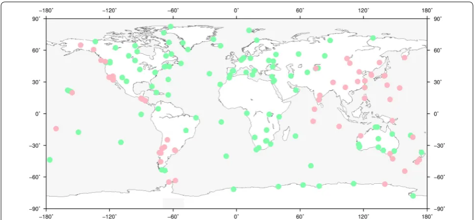
To accurately estimate geocenter motion with GPS data, the site distribution should be globally homog-enous and stable. Thus, the core network of IG2, a well-distributed subset of IGb08 stations, is selected (Fig. 1). This well-distributed sub-network is recommended for the comparison or alignment of global solutions to the IGb08 Reference Frame, since it mitigates the aliasing of stations’ nonlinear motion into transformation param-eters (IGSMAIL-6663: https ://igscb .jpl.nasa.gov/piper mail/igsma il/). Also, for global IGS sites, the core sites are the most stable ones with the longest observation time, which can ensure the reliability of the estimates. Finally, 188 global evenly distributed GPS sites are selected from part of the IGS core sites with high geodetic quality. They satisfy the following criteria: (a) evenly distributed world-wide; (b) continuously observed for at least 10 years; (c) locations far from plate boundaries and deforming zones; and (d) velocity accuracy better than 3 mm/year. Its spatial distribution is shown in Fig. 1. The GPS coor-dinate time series of the selected network can be directly obtained from the IGS SINEX files (ftp://cddis .gsfc.nasa. gov/gps/produ cts/repro 2/). Before applying these data to the geocenter motion inversion, the original coordinate time series have been simultaneously detrended and cor-rected for step discontinuities by least-squares fitting of a linear trend, annual and semiannual sinusoids, as well as
visually obvious offsets terms, at epochs corresponding to equipment changes, and coseismic displacements as reported by ITRF2014 IGS discontinuities file (http://itrf. ensg.ign.fr/ITRF_solut ions/2014/compu tatio n_strat egy. php?page=2). Due to this preprocessing step, our results are not affected by earthquakes.
Theoretically, if the GPS stations are homogenously distributed, the effects of the higher-degree coefficients on GPS-estimated geocenter motion are small. However, an ideal global distributed network is difficult to realize, since no or few data are available around the polar and ocean areas. Therefore, to investigate the aliasing errors of higher degrees, the spherical harmonic load-induced geometrical displacements are truncated with degrees from 1 to 10, respectively.
Results and discussion GPS‑derived geocenter motion
General features of the geocenter estimates
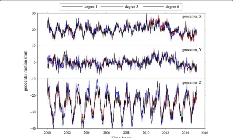
component is obviously higher than those of the X and Y components.
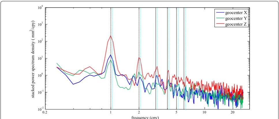
To further understand the periodic signal in GPS-inversed geocenter time series, we compute the power spectral density (PSD) of the geocenter time series with the truncated degree from 1 to 10. The Lomb–Scargle periodogram method is implemented (Deng et al. 2016; Jiang et al. 2014; Williams 2003; Williams et al. 2004). After obtaining the spectra files, all the spectra of the geo-center motion series with truncated degree from 1 to 10 are stacked into one file and then smoothed with a Gauss-ian smoother, so that an overall view of the geocenter motion PSD variations is obtained. Figure 3 presents the final filtered PSD stacking results of the geocenter motion time series inversed from GPS observations. We can see that a dominant annual period with the 1 cycle per year (cpy) frequency is presented in all the three components, among which the Z component have the highest power value, the X component ranks the second, and the Y com-ponent ranks the third. The semiannual signal is relatively weak but is still clear, and the power of the semiannual signals of the X and Y components is less dominated than that of Z component. In addition, the spectra of the stacked GPS-inversed geocenter series show some peaks at the harmonics of the GPS draconitic year (1.04 cpy
harmonics) in all three components, which is also shown in the IG1-inversed results.
Correlations of the GPS geocenter estimates with SLR results To assess the quality of the IG2-inverted geocenter motion, we compare our results with SLR to investigate the correlations of the geocenter estimates obtained from two different space geodesy technologies. We adopt the UT/CSR monthly geocenter time series from the analysis of SLR data based on five geodetic satellites (LAGEOS-1, LAGEOS-2, Starlette, Stella and Ajisai) as reference (ftp://ftp.csr.utexa s.edu/pub/slr/geoce nter/ GCN_RL06_2018_11.txt). Although the SLR ground sta-tions are very sparse and unevenly distributed with only 20 active stations on average, there is also correlated noise existing in the SLR time series, and SLR results still appear to exhibit the most reliable sensitivity to CM due to simpler orbit dynamics and have offered the first competitive geocenter motion result and adopted to estimate the ITRF origin (Altamimi et al. 2016; Riddell et al. 2017; Wu et al. 2017). Considering the data span of SLR and IG2, results from 2002.04107(2002/01/15) to 2015.04107(2015/01/15) are used when comparing this two types of data together.
The left panel of Fig. 4 shows the correlation between SLR and the GPS estimates with translational param-eters coestimated at different truncated degrees. The X-coordinate shows the truncated degrees from 1 to 10. We can see that for all the three components, the geo-center estimates from GPS observations have favorable correlations with SLR results when the truncated degrees are below 6. The highest correlation occurs in the Z com-ponent, while X and Y components have relatively lower correlations. The average values of the correlation coef-ficients for truncated degree from 1 to 6 are 0.35, 0.44 and 0.74 for the X, Y and Z components, respectively. The variations of correlation coefficients from degree 1 to 6 are relatively moderate for all three components.
However, for truncated degrees from degree 7, the cor-relation coefficients of all the three components exhibit obvious decreasing behavior, especially for the X and Z components, implying that the more truncated degrees estimated, the more significant the impact of the aliasing errors of higher degrees in the GPS geocenter motions.
UT/CSR geocenter vector is consistent with IERS con-ventions, approximating the vector from the origin of the TRF to the instantaneous mass center of the Earth (ftp:// ftp.csr.utexa s.edu/pub/slr/geoce nter/READM E_RL06). That is to say, the SLR time series reflects the motion of the CN with respect to the CM, which is not the same as the CM-CF estimates as obtained from the GPS esti-mates. To investigate the effects of the differences in SLR
0.2 1 2 5 10 20
10-2 10-1 100 101 102 103 104
st
ack
ed
pow
er
sp
ect
rum
de
ns
ity
(
mm
2 /cpy)
frequency (cpy)
geocenter X geocenter Y geocenter Z
Fig. 3 Stacked periodogram of the GPS-derived geocenter motion time series with truncated degree from 1 to 10. The blue, green and red lines represent the PSD results of X, Y and Z components, respectively. The black and green vertical dashed lines represent the 1.0 cpy and 1.04 cpy harmonics
Fig. 4 Correlation between SLR and IG2-inverted geocenter motion truncated by different degrees. Blue, green and red lines denote the X, Y and Z
CN-CM data and SLR CF-CM data, we also select the GCN_L1_L2_30d_CN-CM (CN-CM reflects the cor-rection required to best center the SLR network on the geocenter in the absence of modeling any local site load-ing) and GCN_L1_L2_30d_CF-CM (CF-CM is intended to reflect the true degree-1 mass variations without being affected by the higher-degree site loading effects (par-ticularly at the annual frequency)) as references. Results show that the average correlation coefficients between IG2-inverted and the above two SLR geocenter motions for X, Y and Z are 0.20, 0.39 and 0.61 and 0.26, 0.41 and 0.56, which shows overall agreements for SLR results with CF-CM and CN-CM. Therefore, from practical point of view, we think that it is feasible to use UT/CSR CN-CM estimates as reference to evaluate the quality of the IG2-derived geocenter motions.
Seasonal signal analyses
Annual variations
As have been discussed in the above sections, there are obvious seasonal signals (mainly annual and semiannual signals) shown in the GPS-inversed geocenter motions. In this section, we quantitatively compute the variations of the seasonal amplitudes among different truncated degrees and compare these variations with SLR monthly results. Both the annual and the semiannual signals are determined by the unweighted least-squares method with the equation
y(ti)=a+bti+Aacos(2πt−ϕa)+Asacos(4πt−ϕsa) , where a is constant and b represent the trend, Aa and Asa represent the annual and semiannual amplitudes, while ϕa and ϕsa are the corresponding initial phases.
The left panel of Figs. 5 and 6 demonstrates the GPS-derived and SLR obtained annual amplitudes and phases with translational parameters coestimated at truncated degrees from 1 to 10. Compared with SLR results, the GPS-derived annual amplitudes of X and Y components
are smaller, especially for the estimates with truncated degrees 2 and 3. Along with increasing truncated degree, the variations of the GPS-derived annual amplitudes in the X and Y components are stable, among which results with truncated degrees 1, 5 and 10 are much closer to SLR.
With respect to the Z component, the GPS-derived annual amplitudes are higher than the SLR estimates and become increasingly close to the SLR amplitudes until truncated degree 8, among which the estimates with truncated degrees 5 and 8 are much closer to the SLR amplitudes. In terms of the annual phases, results with truncated degree from 4 to 6 have better consistency with SLR for the three components. The X and Y compo-nents exhibit lightly bigger differences for different trun-cated degrees, while the Z component is relatively stable and close to the SLR-estimated phases.
Semiannual variations
Fig. 6 Annual phases of the GPS-derived and SLR obtained geocenter motions with truncated degrees from 1 to 10. The phases of Y component have been shifted 180 degrees. The symbol meanings are the same as Fig. 5. Left: results with translational parameters coestimated, right: results without translational parameters coestimated. Note that in the left panel, the phase angle difference of the X component at 1, 7, 8, 9 and 10 is too big and is not shown in the figure. The situation is the same for the Y component at truncated degree 2
Fig. 7 Semiannual amplitudes of the GPS-derived and SLR obtained geocenter motions with truncated degrees from 1 to 10. Symbols are the same as in Fig. 5. Left: results with translation parameters coestimated, right: results without translation parameters coestimated
the phases of both X and Y components exhibit obvious variation.
From the above correlation and seasonal signal analy-ses, we can see that although the seasonal signals (both the annual and semiannual) of the GPS-inversed geo-center motion vary with different truncated degrees, the estimates with truncated degree 5 are the closest to the SLR geocenter estimates. Therefore, in the follow-ing analysis, the GPS-derived geocenter estimates with translation parameters estimated at the truncated degree 5 are selected as the optimal results.
Non‑seasonal signal analyses
It is already well known that a large part of the geocenter motion comes from seasonal variations. Correspond-ingly, correlations are suspected to indicate how well the seasonality is dominated. To show the agreement of non-seasonal signals, we calculate the correlation of GPS-derived geocenter motion (coestimated with translational parameters) with SLR obtained results after removing the seasonal signals, and the result is shown in the left panel of Fig. 9. We find that the agreement of the non-seasonal signals is relatively weak, with average values of the cor-relation coefficients for truncated degree from 1 to 10 being 0.13, 0.24 and 0.04 for the X, Y and Z components. The GPS-estimated geocenter motions mainly indicate the seasonal signals rather than the non-seasonal signals, respectively. Only the Y component of the non-seasonal GPS geocenter estimates still is consistent with SLR result, indicating that the Y component of GPS results may have some possibility to detect the non-seasonal sig-nals of the geocenter motions, for example the long-term trend.
Comparison between different geocenter estimating approaches
To provide service under the unified and homogeneous reference frame, IGS transforms all the results into the
IGS reference frame (such as IGb08) using Helmert simi-larity transformation after getting solutions from differ-ent analysis cdiffer-enters (ACs, ftp://cddis .gsfc.nasa.gov/gps/ produ cts/repro 2/). The translation parameters are pro-vided as the geocenter estimates in the IGS SINEX files, which refers to the results of the network shift approach. Hereafter, we call it the IG2 sinex solution. To compare our GPS-derived results with results that from the net-work shift approach, we also estimate the seasonal ampli-tudes and phases of the IG2 SINEX solution.
Here we mainly compare the annual signals in this section, just to be consistent with previous researches (Rietbroek et al. 2014; Wu et al. 2015, 2017). The annual amplitudes and phases of the geocenter estimates from different methods are listed in Table 1. According to the conclusion of “Seasonal signal analyses” section, we select the GPS-inversed geocenter motions with truncated degree 5 as our optimal results of the degree-1 deforma-tion approach. We can see that in terms of the annual signals, all three components of the geocenter estimates using the degree-1 deformation approach are better than the results from the network shift approach (compared to slr_itrf2014). Particularly, the amplitude and phase of the Z component obtained from the network shift approach are significantly different from SLR estimates, while the results of the degree-1 deformation approach are very close to those of SLR.
As denoted in “Correlations of the GPS geocenter esti-mates with SLR results” section, the SLR geocenter time series reflect the motion of the CN with respect to the CM, which are not the same as CM-CF. Here, we also list the geocenter motion estimates from SLR contribution to ITRF2014 (referred as slr_itrf2014) (Rebischung et al. 2015) in Table 1. We find that although the amplitudes from slr_itrf2014 are higher in the Y and Z components, the annual phases from slr_itrf2014 are identical to those from slr_GCN_RL06. Therefore, we conclude that the GPS-estimated geocenter motions are consistent with Fig. 9 Non-seasonal geocenter correlations of GPS estimates with SLR results. Blue, green and red lines denote the X, Y and Z components,
SLR results despite the definition differences in the CN and CF.
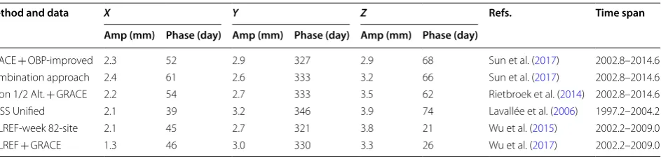
Since GNSS stations are unevenly distributed geo-graphically with sparse coverage in oceanic areas and the Southern Hemisphere, the combination of global GPS data, the assimilated model ocean bottom pres-sure (OBP) models and GRACE data has the potential to provide a complete and independent global measure of spectral mass loading coefficients, including degree one. Therefore, another type of geocenter inverse method is to invert for degree-1 surface mass variation coefficients from various combinations of GNSS observations, OBP models, Jason ocean altimetry and GRACE data (Blewitt and Clarke 2003; Rietbroek et al. 2014; Wu et al. 2015, 2017). To investigate the possible ill-posedness of the GPS loading inversion over sparsely sampled regions such as the ocean, we also compare the geocenter motions esti-mated with combined techniques in terms of annual vari-ations (Table 2). We can see that for the X component, the annual estimates from different approaches correlate quite well in both amplitudes and phases. However, the Y component of the IG2 GPS-derived geocenter motion amplitude is persistently smaller than that of the results derived from other methods, while the Z component of IG2 results has higher annual amplitude. As a whole, the annual phases predicted with the IG2 data are in line with those based on other techniques except that there
is a discrepancy in the Z component, where the IG2-inverted solutions and those obtained from the KALREF approaches are more than one month before those based on other techniques.
Possible reasons for the above differences can be divided into two facets. On the one hand, there exist GNSS observation errors, such as the time-correlated errors in stationdisplacements, remaining draconitic errors in the reprocessed GNSS data, inaccurate or neglected intrinsic variance and correlation structures in the covariance matrices, unmodeled technology-related systematic errors and the truncated higher-degree terms during geocenter motion inversion, etc. Impacts of these factors on parameter estimation, for the most part, are not precisely known right now. On the other hand, inclusion of an OBP model and GRACE data appar-ently improves geographic coverage and the separation of spherical harmonic coefficients (Rietbroek et al. 2014; Swenson et al. 2008; Wu et al. 2015, 2017). However, OBP models generally do not conserve mass or contain accu-rate mass input/output information (i.e., from evapora-tion, precipitation and discharge). They are also built on the static geoid without considering time variable self-gravitation and loading effects of surface mass variations. While these problems can be and have been corrected (e.g., Sun et al. 2017), a more serious concern is that ocean circulation models, even if many oceanographic Table 1 Annual amplitudes and phases of the geocenter coordinate time series from IG2 data and the SLR data
IG2 sinex refers to the network shift approach, and slr_itrf2014 refers to the SLR contribution to the ITRF2014 (Rebischung et al. 2015)
Method and data X Y Z
Amp (mm) Phase (day) Amp (mm) Phase (day) Amp (mm) Phase (day)
IG2 estimates 2.2 55 1.3 332 5.3 32
IG2 estimates without trans. 2.1 43 1.3 278 5.8 31
IG2 sinex 1.4 42 3.6 306 3.6 170
slr_GCN_RL06 2.7 55 2.1 321 5.0 29
slr_itrf2014 2.6 48 2.8 320 5.9 26
Table 2 Estimated amplitudes and phases of the annual variations of the geocenter motions obtained from different combination approaches
Method and data X Y Z Refs. Time span
Amp (mm) Phase (day) Amp (mm) Phase (day) Amp (mm) Phase (day)
vations from IG1 are adopted to inverse the geocenter motions. The same analyses as the IG2 are then imple-mented to the IG1 solutions so as to investigate the pos-sible improvements. Considering that the IG1 data span ended in early 2010, we compare results from 2002.04107 to 2009.95547. Figure 10 represents the geocenter corre-lations of the IG1 and the SLR results together with the annual signal comparison with (left panels) and without (right panels) coestimating the translation parameters. Generally, the IG1 estimates with truncated degree 4 are the closest to the SLR results. The average values of the correlation coefficients with SLR results for IG1 are 0.58, 0.48 and 0.66 for the X, Y and Z components, while for IG2 results within the same time span, the mean values are 0.42, 0.46 and 0.75. The correlations of the X compo-nent for IG1 are better than IG2, but Z component exhib-its worse correlations. On the whole, the estimates with the truncated degree 4 are the closest to the SLR geo-center estimates. Compared to IG2 estimates, although the IG1-derived annual amplitude of the Y component is more consistent with SLR estimates, its annual phase is far away (nearly two month apart) from SLR. There is no optimal truncated degree for both the annual amplitudes and phases that are consistent with the SLR. This indi-cates the IG2 improvements over the previous IG1 repro-cessing efforts (see details at http://acc.igs.org/repro cess2 .html). We also find that the IG1 geocenter estimates without coestimating the translational parameters show more moderate variations, but exhibit obvious discrep-ancies with the IG1 results with translational parameters coestimated.
Effects of the translational parameters in the inversion model
As mentioned in “Method and data” section, we find that there are three translation parameters ( (tx ty tz) ) in the functional model of the degree-1 deformation approach. However, there are no agreements about whether the translational parameters should be estimated. In this sec-tion, we investigate the effects of the translational param-eters on the IG2-inversed geocenter motions. For clear comparison, the right panel of Figs. 4, 5, 6, 7, 8 and 9
amplitudes with truncated degree 5 is the closest to the SLR amplitudes for all three components, while for the annual phases with different truncated degrees, only Z components show little differences and are always close to the SLR-estimated phases. The most significant varia-tions with and without coestimating translational param-eters appeared in the Y component. When the truncated degree is 1, the annual phase of Y component is close to the SLR. However, if truncated at degree 2, the phase became 30° larger than the SLR results. If the truncated degrees are between 3 and 10, the phases become stable and are approximately 45° smaller than the SLR results. For the X component, the annual phases with truncated degree from 3 to 6 have better consistence with SLR.
In total, despite the fact that the variations of correla-tion coefficients from different degrees without transla-tional parameters coestimated are more moderate than results with translational parameters coestimated, for every truncated degree, big discrepancy exists in the annual signal estimates between the GPS-derived results without translational parameters coestimated and the SLR results. Therefore, the GPS geocenter motion esti-mated with translational parameters demonstrates more positive results than that without translation parame-ters. Thus, we propose that the translational parameters should be considered when estimating geocenter motion with the IG2 core stations’ coordinate time series.
Effect of the post‑seismic deformation
the X component with truncated degree bigger than 7 and the Y component. Except for the solutions with trun-cated degree 3, the amplitudes of Y component are higher than those of the SLR results, and the average value of the annual amplitudes of the Y component for trun-cated degree from 1 to 10 is 3.3 mm, which is very close to results derived from other methods (Table 2). With respect to the annual phases, results for both the X and Z components indicate the same variations as from the 186 station solutions. The only significant difference occurs
in the Y component. Except for the results with trun-cated degree 3, the annual phase of the Y component is nearly three month apart from SLR estimates. Therefore, we conclude that after removing the stations affected by large earthquakes, the amplitudes of Y component do become higher, but the annual phases of the Y compo-nent become far away from the SLR results. We also find that without coestimating the translational parameters, the geocenter estimates show nearly the same results as solutions from the 186 stations.
An equivalent water height map of the estimated SH coefficients
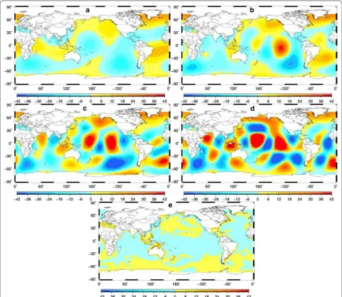
As mentioned in “Comparison between different geo-center estimating approaches” section, the lack of the GPS stations in oceanic areas can lead to unstable solu-tions when inversing global measure of spectral mass loading coefficients, including degree one. In order to declare this ill-posedness, we create an equivalent water height (EWH) map from the IG2-estimated SH coeffi-cients (including higher-order terms) and compare the results with the solutions provided by the Estimation of the Circulation and Climate of the Ocean (ECCO). The
SH coefficients from 2008/04 (2008 April) are adopted to compute the equivalent water height to check whether the ocean values obtain reasonable physical values. Fig-ure 12 illustrates the results from SH coefficients with truncated degree at 5, 7, 9, 10 (a–d) as well as the ECCO solutions (e). We can notice that the differences between IG2 SH coefficients and ECCO solutions vary with dif-ferent truncated degrees. Despite the fact that the IG2 coefficient-inversed EWH with truncated degree 5 is most closely to ECCO solutions, there are still obvious differences occurring in northern and central Atlantic Ocean areas, as well as the central Indian Ocean areas. Fig. 11 Geocenter correlations and the annual estimations of the IG2-inversed geocenter motions after removing the stations affected by
With the truncated degree grows, the differences become more and more significant, and the consistency between the two different types of solutions is getting worse and worse. Therefore, to obtain stable geocenter motions from the global GPS data, and to expand GPS to inverse the global surface mass loading displacements, further researches still need to be done to combining the OBP models, as well as other datasets (Rietbroek et al. 2014; Sun et al. 2017).
Conclusions
SLR results. The average values of the correlation coef-ficients with truncated degree from 1 to 6 are 0.35, 0.44 and 0.74 for the X, Y and Z components, respectively. For truncated degrees from degree 7, the three components exhibit obvious decreasing variations, especially for the X and Z components, implying that with more truncated degrees estimated, there is more significant impact of the aliasing errors of higher degrees on the GPS-derived geo-center motions.
Our stacked periodic analysis of the GPS geocenter estimates indicates that a dominant annual period with the 1 cpy frequency is presented in all three components, while the semiannual signal is relatively weak. The annual amplitudes of X and Y components are relatively smaller than SLR results, and the variations are stable with dif-ferent truncated degrees. However, the amplitudes of the Z component of the inversed geocenter are higher than SLR. In terms of the annual phases, the X and Y com-ponents show bigger differences for different truncated degrees, while the Z component is relatively stable and close to the SLR-estimated phases. For all the three com-ponents, the GPS geocenter estimates with truncated degree 5 are the closest to the SLR estimates. Besides the periodic analysis, we also carry out non-seasonal analy-sis for the IG2-inverted and the SLR obtained geocenter motion. Results show that the Y component of the resid-ual GPS geocenter estimates still correlates with SLR.
Then, the GPS-derived geocenter motions are com-pared with results from other different geocenter esti-mating approaches. For both annual amplitudes and phases, geocenter estimates obtained from the degree-1 deformation approach are better than results from the network shift approach using the same GPS data. They are also very consistent with the SLR RL06 results and the geocenter estimates from the SLR contribution to the ITRF2014. As a whole, the annual phases predicted with the IG2 data are in line with those based on other combination techniques. An exception is that there is a discrepancy in the annual phase estimates of the Z com-ponent. We find that solutions based on IG2 data, as well as those based on the KALREF approaches, are more
over the previous IG1 reprocessing efforts.
Furthermore, the effects of the translational param-eters are investigated. In terms of the annual geocenter motion estimates, for every truncated degree, big dis-crepancy exists in the annual signal estimates between the GPS-derived results without translational param-eters coestimated and the SLR results. The most sig-nificant variations appear in the Y component, which is approximately 45 days apart from the SLR results with different truncated degrees for results without transla-tional parameters coestimated. Thus, we propose that the translational parameters should be considered when estimating geocenter motion with the IG2 core stations’ coordinate time series.
Additional file
Additional file 1. IG2 derived geocenter data.
Acknowledgements
We are grateful to the International GNSS Service (IGS) for providing the origi-nal data sets. Also many thanks to the editor and JEO assistant for important suggestion in the manuscript processing. We thank the two anonymous reviewers for their constructive comments and suggestions, which help to improve the manuscript significantly.
Authors’ contributions
All the authors contributed to the design of the study. LD came up with the idea of the study. LD, ZL and YM carried out the experiments and drafted the manuscript. NW and HC participated in the experimental analysis. All authors read and approved the final manuscript.
Funding
This research is supported by the National Science Fund for Distinguished Young Scholars (No. 41525014), together with the Scientific Research Project of Hubei Provincial Department of Education, Surveying and Mapping Basic Research Program of the National Administration of Surveying, Mapping and Geoinformation (No. 17-01-01) and Research Program of Hubei Polytechnic University (No. 18xjz09R).
Availability of data and materials
The coordinate products from IGS are available at FTP site: ftp://igs.ign.fr/pub/ igs/produ cts/$WEEK/repro 2/. The SLR data can be downloaded in ftp://ftp.csr. utexa s.edu/pub/slr/geoce nter.
Ethics approval and consent to participate Not applicable.
Consent for publication Not applicable.
Competing interests
The authors declare that they have no competing interests.
Author details
1 Optics Valley BeiDou International School, Hubei Polytechnic University, 16
Guilinbei Road, Huangshi 435003, China. 2 Department of Land Surveying
and Geo-Informatics, The Hong Kong Polytechnic University, 181 Chatham Road South, Hung Hom, Kowloon 999077, Hong Kong, China. 3 GNSS Research
Center, Wuhan University, 129 Luoyu Road, Wuhan 430079, China. 4 IGN
LAREG, Université Paris Diderot, Paris, France. 5 School of Geodesy and
Geo-matics, Wuhan University, 129 Luoyu Road, Wuhan 430079, China.
Received: 9 November 2018 Accepted: 26 June 2019
References
Altamimi Z, Rebischung P, Métivier L, Collilieux X (2016) ITRF2014: a new release of the international terrestrial reference frame modeling nonlinear station motions. J Geophys Res Solid Earth 121(8):6109–6131
Argus DF (2012) Uncertainty in the velocity between the mass center and surface of earth. J Geophys Res Solid Earth 117(B10405):1–15 Blewitt G (2003) Self-consistency in reference frames, geocenter
defini-tion, and surface loading of the solid earth. J Geophys Res Solid Earth 108(B2):2103–2013
Blewitt G, Clarke P (2003) Inversion of Earth’s changing shape to weigh sea level in static equilibrium with surface mass redistribution. J Geophys Res (Solid Earth) 108:2311. https ://doi.org/10.1029/2002J B0022 90
Blewitt G, Lavallée D, Clarke P, Nurutdinov K (2001) A new global mode of earth deformation: seasonal cycle detected. Science 294(5550):2342–2345
Bloßfeld M, Seitz M, Angermann D (2014) Non-linear station motions in epoch and multi-year reference frames. J Geod 88(1):45–63
Chambers DP, Tamisiea ME, Nerem RS, Ries JC (2007) Effects of ice melting on grace observations of ocean mass trends. Geophys Res Lett 34(5):5610 Cheng MK, Ries JC, Tapley BD (2013) Geocenter variations from analysis of SLR
data. In: Altamimi Z, Collilieux X (eds) Reference frames for applications in geosciences. International association of geodesy symposia, vol 138. Springer, Berlin, Heidelberg
Collilieux X, Altamimi Z, Ray J, Dam TV, Wu X (2009) Effect of the satellite laser ranging network distribution on geocenter motion estimation. J Geophys Res Solid Earth 114(B4402):1–17
Collilieux X, Van Dam T, Ray JR, Coulot D, Metivier L, Altamimi Z (2012) Strate-gies to mitigate aliasing of loading signals while estimating GPS frame parameters. J Geod 86(1):1–14
Deng L, Jiang W, Li Z, Chen H, Wang K, Ma Y (2016) Assessment of second- and third-order ionospheric effects on regional networks: case study in China with longer CMONOCGPS coordinate time series. J Geod 91(2):1–21 Dong D, Dickey JO, Chao Y, Cheng MK (1997) Geocenter variations caused
by atmosphere, ocean and surface ground water. Geophys Res Lett 24(15):1867–1870
Dong D, Fang P, Bock Y, Cheng MK, Miyazaki S (2002) Anatomy of apparent seasonal variations from GPS-derived site position time series. J Geophys Res Solid Earth 107(B4):ETG-1-ETG 9-16
Dong D, Qu W, Fang P, Peng D (2014) Non-linearity of geocentre motion and its impact on the origin of the terrestrial reference frame. Geophys J Int 198(2):1071–1080
Farrell WE (1972) Deformation of the earth by surface loads. Rev Geophys 10(3):761–797
Feissel-Vernier M, Bail KL, Berio P, Coulot D, Ramillien G, Valette JJ (2006) Geocentre motion measured with DORIS and SLR, and predicted by geophysical models. J Geod 80(8–11):637–648
Ferland R, Piraszewski M (2009) Theigs-combined station coordinates, earth rotation parameters and apparent geocenter. J Geod 83(3–4):385–392 Fritsche M, Dietrich R, Rülke A, Rothacher M, Steigenberger P (2010)
Low-degree earth deformation from reprocessed GPS observations. GPS Solut 14(2):165–175
Jiang Weiping, Deng Liansheng, Li Zhao, Zhou Xiaohui, Liu Hongfei (2014) Effects on noise properties of GPS time series caused by higher-order ionospheric corrections. Adv Space Res 53(7):1035–1046
Jin S, Dam TV, Wdowinski S (2013) Observing and understanding the earth system variations from space geodesy. J Geodyn 72(12):1–10 Kang Z, Tapley B, Chen J, Ries J, Bettadpur S (2009) Geocenter variations
derived from GPS tracking of the grace satellites. J Geod 83(10):895–901 Lavallée DA, Dam TV, Blewitt G, Clarke PJ (2006) Geocenter motions from GPS:
a unified observation model. J Geophys Res Solid Earth 111(B05405):1–15 Lavallée DA, Moore P, Clarke PJ, Petrie EJ, van Dam T, King MA (2010) J2: an
evaluation of new estimates from GPS, grace, and load models compared to SLR. Geophys Res Lett 37(22):707–716
Meindl M, Beutler G, Thaller D, Dach R, Jäggi A (2013) Geocenter coordinates estimated from GNSS data as viewed by perturbation theory. Adv Space Res 51(7):1047–1064
Melachroinos SA, Lemoine FG, Zelensky NP, Rowlands DD, Luthcke SB, Bordyu-gov O (2013) The effect of geocenter motion on Jason-2 orbits and the mean sea level. Adv Space Res 51(8):1323–1334
Petit G, Luzum B, Al E (2010) IERS conventions (2010). IERS Tech Note 36:1–95 Rebischung P et al (2015) Repro2 TRF combinations: combination of the IGS repro2 terrestrial frames a poster presentation at the 2015 European Geosciences Union
Rebischung P, Altamimi Z, Springer T (2014) A collinearity diagnosis of the GNSS geocenter determination. J Geod 88(1):65–85
Rebischung P, Altamimi Z, Ray J, Garayt B (2016) Theigs contribution to ITRF2014. J Geod 90(7):611–630
Riddell AR, King MA, Watson CS, Sun Y, Riva R, Rietbroek R (2017) Uncertainty in geocenter estimates in the context of ITRF2014. J Geophys Res 122(5):4020–4032
Rietbroek R, Fritsche M, Brunnabend SE, Daras I, Kusche J, Schröter J et al (2012) Global surface mass from a new combination of grace, modelled OBP and reprocessed GPS data. J Geodyn 59–60(5):64–71
ing effects in the inversion for load coefficients and geocenter motion from GPS data. Geophys Res Lett 29(24):63-1–63-4
Wu X, Ray J, Dam TV (2012) Geocenter motion and its geodetic and geophysi-cal implications. J Geodyn 58(3):44–61
Wu X, Abbondanza C, Altamimi Z, Chin TM, Collilieux X, Gross RS et al (2015) KALREF—a Kalman filter and time series approach to the International Terrestrial Reference Frame realization. J Geophys Res 120(5):3775–3802