Blind estimation of statistical properties of non stationary random variables

R E S E A R C H

Open Access

Blind estimation of statistical properties of

non-stationary random variables

Ali Mansour

, Raed Mesleh

and el-Hadi M Aggoune

Abstract

To identify or equalize wireless transmission channels, or alternatively to evaluate the performance of many wireless communication algorithms, coefficients or statistical properties of the used transmission channels are often assumed to be known or can be estimated at the receiver end. For most of the proposed algorithms, the knowledge of transmission channel statistical properties is essential to detect signals and retrieve data. To the best of our knowledge, most proposed approaches assume that transmission channels are static and can be modeled by

stationary random variables (uniform, Gaussian, exponential, Weilbul, Rayleigh, etc.). In the majority of sensor networks or cellular systems applications, transmitters and/or receivers are in motion. Therefore, the validity of static

transmission channels and the underlying assumptions may not be valid. In this case, coefficients and statistical properties change and therefore the stationary model falls short of making an accurate representation. In order to estimate the statistical properties (represented by the high-order statistics and probability density function, PDF) of dynamic channels, we firstly assume that the dynamic channels can be modeled byshort-term stationary but long-term non-stationary random variable (RV), i.e., the RVs are stationary within unknown successive periods but they may suddenly change their statistical properties between two successive periods. Therefore, this manuscript proposes an algorithm to detect the transition phases of non-stationary random variables and introduces an indicator based on high-order statistics for non-stationary transmission which can be used to alter channel properties and initiate the estimation process. Additionally, PDF estimators based on kernel functions are also developed. The first part of the manuscript provides a brief introduction for unbiased estimators of the second and fourth-order cumulants. Then, the non-stationary indicators are formulated. Finally, simulation results are presented and conclusions are derived.

Keywords: Wireless communication; Dynamic transmission channel; Higher-order statistics; Cumulants; Cumulative distribution function; Kernel density estimators; Hermite basis set; Spline functions; Characteristic functions;

Non-stationary signals

1 Introduction

Unlike discrete transmission channels which have limited practical value, continuous random transmission chan-nels are widely accepted and used to illustrate practical concepts [1]. In numerous proposed algorithms, statis-tical properties or probability density function (PDF) of transmission channels are assumed to be perfectly known or already estimated [2-6]. To analyze the perfor-mance of various wireless transmission schemes, Simon and Alouini in [7] have used channel statistical models and PDF properties. It is widely believed that wireless

*Correspondence: [email protected]

1LAb STIC - ENSTA Bretagne, 2 Rue François Verny, Brest 29200, France Full list of author information is available at the end of the article

transmission channels can be modeled using stationary random variables [1,8,9]. We should highlight the fact that various PDFs have been used in the context of wireless communications, such as Gausssian, Rayleigh, log-normal, exponential, one-sided Gaussian distribution, Hoyt, Weibull, Rice, Nakagami-m,α−μ, andη−κ (see [10-21] and the references therein). It is worth pointing out that parametrical estimation methods can be used if the channel model (or a PDF for the real random variable (RV)) is selected or identified. Additionally, non-parametrical estimation methods can also be found in the literature [22-27]. However, these methods are hard to be implemented and mostly time consuming and they strongly relate to the proposed models and applications. For this main reason, a generic method and few required

assumptions about the transmission channel are proposed and discussed in this manuscript.

The recent spread of cellular systems (smart sen-sors, mobile phones, base stations, satellites, surveillance devices, traffic radars, etc.) has increased the complexity of processing algorithms as well as the model of transmis-sion channels. In fact, in various applications, transceiver units are in motion. For such systems, the transmission channels can no longer be considered as static chan-nels, i.e., they cannot be modeled by stationary random variables. To overcome this difficulty, most researchers assume that the transmission channels are static during the processing timea[28-30].

In this manuscript, the proposed models are improved by considering that transmission channels are dynamic channels that can be modeled as non-stationary vari-ables. It is worth mentioning that for antennas mounted on moving vehicles or drones, the transmission channels can be approximated by almost static or slowly evolution-ary dynamic channels over certain periods. The transition among these periods can be very fast. In addition, dur-ing two adjacent periods, transmission channels can have completely different statistical properties and/or PDFs. This scenario illustrates a typical scenario of a mobile phone used in a moving car which is moving among big buildings in a modern city. It can represent as well the sce-nario of a drone flying at low altitude in a mountainous area.

In what follows, we consider that transmission chan-nels can be modeled as short-term stationary signals and long-term non-stationary signals (many natural and physical signals belong to this category, such as speech signals [31,32]). Herein, we develop an algorithm to accu-rately estimate the transition times. The algorithm is based on high-order statistics (HOS). In several study cases, HOS are shown to be more promising than the second-order stochastic methods, namely, power, vari-ance, covarivari-ance, and spectra. In fact, HOS have been used to solve many recent and important telecommuni-cation problems [33,34], such as blind identifitelecommuni-cation or equalization, blind separation of sources, and time delay estimation [35-38]. It is worth mentioning that most of these HOS algorithms are only based on the second- and the fourth-order statistics [39]. Once the transition times are estimated, we should be able to estimate the PDF of the local stationary random variable (i.e., during a short-term period).

It is well known that any random variable can be com-pletely described by its PDF [40]. In many cases, an accurate estimation of the PDF of physical parameters of interest (which are random variables) is essential to achieve our goals. This is while an accurate estimation of PDFs is still challenging to researchers. The estima-tion of PDFs is a relatively old problem that has been

considered since the beginning of the last century with the rise and the development of new and modern com-plex systems (radars, sonar, and wireless communication systems). However, in late 1950s, systematic mathemati-cal approaches have been proposed. One of the pioneering work in this field is the work presented by Rosenblatt in [41]. Parzen in [42] formulated the estimation of PDFs using kernel approaches. Later on, new approaches emerged to overcome the specification of diverse appli-cations such as the sum of Gamma densities in Risk Theory [43] or the sum of exponential random variables in wireless communication [44]. Other researchers have focused on the choice of the kernel and smoothing func-tions [45,46]. The estimation of PDFs using orthogonal series has been introduced by Schwartz in [47]. In more recent work, wavelets have been used as a non-parametric estimation of PDFs [48]. Similar to previous work, Engel used Haar’s series to estimate PDFs [49]. Using autore-gressive (AR) models, Kay in [50] proved that PDFs can be estimated by appealing the theory of power spectral density (PSD). More recent work reintroduced the estima-tion of PDF using a windowed Fourier transform [51] or Hermite’s orthonormal basis set [52]. We should mention that all the abovementioned work assume that the random variables are stationary. In countless applications, the sta-tionarity assumption may be invalid [53]. To the best of our knowledge, there is no such PDF estimator for non-stationary random variables. Hence, it is the aim of this paper to propose a PDF estimator based on a smooth ker-nel PDF estimator that assumes known transition times.

2 Mathematical model and background

In this paper, we consider the case of real non-stationary random variablesb. We also assume (1.1 in Appendix 1) that random variables consisting of transmission chan-nels are stationary by part [54,55]. While this assump-tion is less strict than the most widely used assumpassump-tion of stationary transmission channels, its consideration is justified in the case of moving receivers or transmitters.

Hereinafter, Pr(A) stands for the probability of the event A. Letx1,. . .,xn stand forn independent

realiza-tion of a continuous RV X. In addition, let us denote by

fX(x),FX(x),fˆX(x), andFˆX(x)respectively as the PDF, the

cumulative distribution function (CDF) of X, and their estimated functions:

FX(x)=Pr(X≤x)=

_x

−∞fX(x)dx. (1) In the following,k(x)denotes a kernel function ofx, and the mathematical expectation (i.e., the mean) of a real RV

Xis denoted by

mX=E{X} =

whereEstands for the mathematical expectation. By defi-nition [56], theqth-order momentμqof a stochastic signal Xis

We mentioned earlier that a real random variableXis completely described by its PDFfX(x). In addition, a

ran-dom variable can also be described by its first_X(u)or second_X(u)characteristic functions as follows:

X(u) = E{ejXu} =

wherej2 = −1. While the second characteristic function can be directly obtained from the first one, the first one is considered as the inverse Fourier transform of the PDF. Theoretically, PDFs may be obtained by the Fourier trans-form ofX(u). The Taylor series of the two characteristic

functions yield other important statistical functions which are the moments and the cumulants [56]:

mk(X) = E{Xk} = (−j)k∂

According to the theorem of Leonov-Shiryayev [56], therth-order cumulant of X can be calculated from its moments, using the following formulac[53,57]:

Cumr[X]=Cum[X,. . .,X]

=(−1)k−1_(k−1)!E[Xv1_]E[Xv2_]. . ._E[Xvp_]. (8)

Using this relationship, we can evaluate the fourth-order cumulant ofXas

Cum4[X]=E[X4]−4E[X]E[X3]−3E2[X2]+12E2[X]E[X2] −6E4[X] .

(9)

For a zero-mean stochastic signal (please see [58] and the cited references therein),dthe second-order cumulant is equal to the second-order moment and therefore the fourth-order cumulant becomes

Cum4[X]=E[X4]−3E2[X2] . (10)

The HOS are much easier to be estimated than PDF, as will be shown in the next section. For this reason, our non-stationary transition indicator is based on the

second-and fourth-order statistics. In fact, the transition of non-stationary random variable can generate discontinuity in its HOS. As the variance of any signal should be different than zero, then it can be used to identify the existence of signals. On the other hand, normalized signals have the same unit variance. Therefore, the variance is not enough to identify the transition in a general case. Besides that, the fourth-order cumulants of Gaussian signals are zeros. For these reasons, we developed a non-stationary transi-tion indicator based on the variance and the fourth-order cumulant.

3 Unbiased and adaptive HOS estimators

LetXbe a zero-mean stochastic signal wherexiis an event

(or a signal sample) ofX(1≤i≤N). The classic estimator of therth-order moment ofXis given by

It is easy to verify that (11) is an unbiased estimator of therth-order moment ofX(i.e.,E[μ_r]= μ_r). To esti-mate the fourth-order cumulant of X, we can derive an estimator from the Leonov-Shiryayev formula (8):

Cum4[X]=μ4−3μ22. (12)

It is established [59,60] that the estimator in (12) is a biased estimator and the estimation error decreases proportional to_N1. In fact, using (11) and (12) we can write

and the estimator expectation becomes

E[Cum4[X]]=μ4−

Using the Leonov-Shiryayev formula, one can develop an unbiased estimator for the cumulant ase

Let μr{k} be the estimator of the rth-order moment at the kth iteration, and we can develop the following adaptive estimators for the second- and the fourth-order statistics:

for 1<k≤N. This algorithm is simple and converges quickly in the case of stationary signals. Another adaptive estimator of a fourth-order cross-cumulant (Cum13(X,Y)) which is more suitable for non-stationary

signals is given by

CN =N−

where 0< γ <1 is another forgetting factor.

4 PDF estimators

To get an accurate estimation of fX(x), one should use

available observations or measurements (i.e., x1,. . .,xn).

Using Fubini’s theorem [61]f, Rosenblatt in [41] proved that any estimatorfˆX(x) of fX(x) based on the set ofxi,

where Card denotes the cardinal of aσ-algebra set. Using the fact thatfX(x)= dFX_dx(x), Parzen proposed an

asymptot-ically unbiased estimator of the PDF as the sum of scaled and shifted kernel functions:

fn(x)=

are Borel’s functions [62]g in L1 function space, which satisfy few conditions such as [41,47]

Rk(x)=1.

In [42], Parzen suggests few kernel functions including histograms which are kernel estimators when

k(x)= u(x+1)−u(x−1)

2 ,

withu(x)being the Heaviside step function.

Using the definition in (4), the PDFfX(x)can be

approx-imated by using the Fourier transform of an estapprox-imated characteristic function [53]. In fact, the average over a set of realization is an unbiased estimator of the mathe-matical expectation of a RV. Therefore, the first charac-teristic function can be approximated using the following equation:

In [51], the authors mentioned that the Fourier trans-form of the last equation cannot converge. However, it is possible to obtain the Fourier transform of the product betweenˆ_X(u)and a weighting windoww(x). In this case the PDF estimator is given by

ˆ

The above equation can be considered as a kernel esti-mator. Window length and parameters are the key factors which can affect the performance of the estimator [51]. To avoid the problem of this approach and apply the well-established theory of power spectral density, Kay in [50] proposed an AR model of order p to estimate the PDF. Parameters of his AR model are estimated using Yule-Walker equations and Levinson recursion.

Using Gram-Charlier series to expand the PDF in terms of the normal density and its derivatives, Bowers in [43] approximated a risk theoretic distribution by the sum of Gamma RVs. In his expansion, the polynomials which multiply the PDF of a zero-mean normalized normal PDF are the Hermite polynomials (see Appendix 2). This study was generalized by Schwartz in [47].

mean square error. In real-world applications, another problem can arise related to the evaluation of the scal-ing and the mother functions at arbitrary points [24]. In [49], Engel used Haar’s functions to estimate the PDF and shows that his estimator is equivalent to a histogram on certain dyadic intervals.

Recently, the authors of [51,52] have compared their approaches to the abovementioned ones. In fact, Xie and Wang in [51] showed that an estimator based on the Fourier transform of the characteristic function gives sim-ilar results to the AR model PDF estimator proposed earlier by Kay in [50]. They also showed that in certain cases, histograms can provide similar overall performance to previously mentioned estimators. However, Howard in [52] showed that the Hermite basis estimator can slightly achieve better results than the estimator based on the Fourier transform of the characteristic function proposed in [51]. For these reasons, we only consider the histogram, the Hermite basis estimator and the smooth kernel density estimator proposed by Bowan in [45,46]. Our simulations have shown that smooth kernel density has slightly bet-ter performance than the previous mentioned ones (see Section 7).

Finally, two useful error measures are proposed to evaluate the overall performance of various estimators [41,47,51,52]:

- The integrated error

1=E{|fX(x)− ˆfX(x)|}

- The root of the mean-squared error

2=

E{|fX(x)− ˆfX(x)|2}

5 Representation of non-stationary PDF

Real-world signals can be modeled by wide or quasi non-stationary random variables [39,63]. In this case, the PDF is a time-dependent functionfX(x,t)wheretcan be a

vec-tor representing discrete time instants. Let us consider for example a wireless transmission channelh(t)which can be modeled by a quasi stationary RV [1]. Let us assume now thath(t)has a Weibull PDF for the first period, a uniform PDF for the second period, then a Gaussian RV in its last parts. In this case, it becomes clear that the PDF ofh(t)

cannot be represented by simple curve as function oftor

X. Hence, the PDF of non-stationary RV should be plotted as a function of a RVXandt(see Figure 1).

In fact, classic PDF estimators cannot provide an accu-rate estimation of the non-stationary signal PDF. By applying a smooth kernel density estimator over 10,000 independent realization of h(t), a bimodal PDF was

obtained (see Figure 1b). It is clear that the obtained PDF cannot correctly represent the PDF shown in Figure 1a.

6 Non-stationary transition indicator

In order to estimate the PDF parts of quasi non-stationary RV, one can easily use the estimator developed in the pre-vious section to detect the number and the size of the stationary parts. Once these parts are well identified and their sizes are relatively enough to estimate a PDF, we can apply any classic PDF estimator. To make this esti-mation more robust, cumulants of different order (mainly the second and the fourth order) can be used to iden-tify such parts. In fact, Gaussian signals are characterized by their zero fourth-order cumulant (see Appendix 1). In these case, the fourth order cannot separate two adjacent Gaussian parts. However, if these two parts represent two normal RVs with different means or variances, then the second or the first moment can be used to identify these parts. If the two Gaussian parts have the same mean and variance then they can describe the same RV due to the basic assumptions about the whiteness of the samples (i.e., the realization ofX).

Hereinafter, we consider that the non-stationary RV is formed by successive segments of stationary RV. In order to estimate the PDF of the non-stationary signal, an esti-mator of the transition times should be developed. In order to simplify our discussion and gain insight, a generic case is considered. Let us consider a zero-mean non-stationary signal X(t) made by four parts of stationary random variables as shown in Figure 2:

1. The first part contains 8,000 samples of uniform random variable included in[−1, 1].

2. The second part is made of 6,000 samples of zero-mean and unite variance Gaussian signal. 3. The 10,000 samples of a uniform random variable in

[−2, 2]formed the third part.

4. The fourth part is a zero-mean Gaussian signal with a standard deviation of√2.

The fourth-order statistics of the uniform parts are given as follows:

E[X2] = A

2

3 ,

E[X4] = A

4

5 ,

Cum4[X] = −

2A4

15 , (19)

0 1 2 3 4 5 0

0.1 0.2 0.3 0.4 0.5 0.6 0.7 0.8

t fX

(x,t)

(b)

(a)

Figure 1Theoretical and estimated PDF of non-stationary RV.The estimation is done using smooth kernel density estimators.(a)Theoretical PDF.(b)Estimated PDF.

noisy signals. To reduce the noise level, we adopted two steps:

1. First, the obtained signals are filtered using the smoothing polynomial regression filter proposed by Savitzky-Golay [64-66]. The main idea of the Savitzky-Golay filter is to apply a FIR filter such that its coefficients minimize the mean-squared

approximation error. This filter is used to filter biomedical signals such as EEG signals (see Figure 4). 2. Second, the noise in the filtered signals are slightly

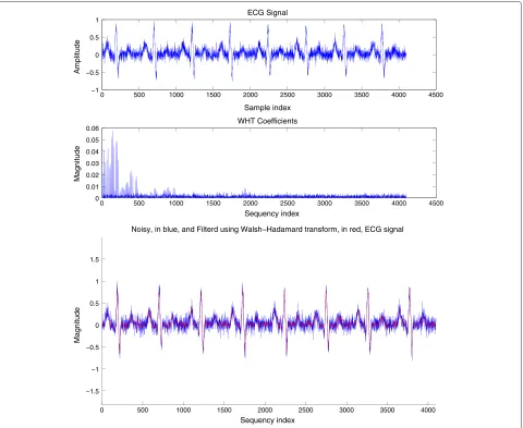
reduced using a Walsh-Hadamard transform which is a generalization of discrete Fourier transform [67]. This transformation is also used in biomedical signals to filter and compress ECG signals (see Figure 5).

In order to smooth the HOS estimator and achieve bet-ter detection of the transition times, the signal of the HOS estimator was firstly filtered using a Savitzky-Golay filter then a Walsh-Hadamard transform truncation fil-tering techniques is applied. Experimental results showed

that the filtered signals are much more smooth and useful to reach our goal (see Figure 6).

While the filtered signals are much better smoothed than the raw signals, they are still relatively noisy to obtain an accurate estimate of transition time. In fact, Figure 6 shows that the obtained filtered estimators are still suf-fering from the previously mentioned drawbacks, i.e., the inaccuracy in the estimation of the HOS and the transition times.

To address the previously mentioned problems, we developed the following algorithm:

- First, the PDF of the filtered HOS estimators are obtained using the kernel PDF estimator (see Figure 7). Then the maximum values of the obtained PDF are recorded as the coefficients of a vector called maxHOS.

- The coefficients of the vector maxHOS are introduced as the center of clusters. By minimizing Euclidean distance among the samples of the filtered HOS estimator, all samples of filtered estimated

0 0.5 1 1.5 2 2.5 3 3.5

x 104

−8 −6 −4 −2 0 2 4 6

Non−Stationary Signal

0 0.5 1 1.5 2 2.5 3 3.5

x 104 _{x 10}4

0 1 2 3 4 5 6

Theorirical and Estimated Variance

0 0.5 1 1.5 2 2.5 3 3.5

−50 −40 −30 −20 −10 0 10 20

Theortical and Estimated Cummulants

Figure 3Theoretical and estimated values of variances and fourth-order cumulants of non-stationary signals.

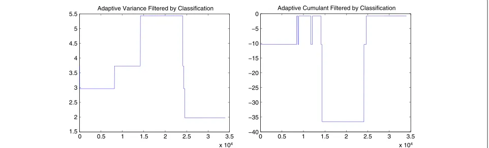
cumulants are clustered in rectangular signals which represent theoretical values of the HOS (see Figure 8). - Various simulations have been conducted. Our

simulations showed that sometimes the rectangular clustered signals suffer from local narrow spurious error windows (see Figure 8). These spurious error windows are normally very narrow. Hence, by supposing that the channel is not a highly dynamic one, i.e., any channel parameter cannot change more than one time in a short period (for example, the short period can be the symbol duration). In this case, one can easily eliminate these windows. In order to clean out the clustered rectangular signals and achieve an accurate non-stationary indicator, the derivative of these signals is evaluated (see Figure 9). - Let us assume 1.2 in Appendix 1 that the stationary

parts of the channels have more than 1,000 samples (in many cases, 500 samples were enough to obtain

0 500 1000 1500 2000 2500 3000 3500 4000

−2 0 2 4 6 8 10 12

Noisy, in blue, and Filterd using Sgolay filter, in red, ECG signal

Sequency index

Magnitude

Figure 4A fifth-order Savitzky-Golay filter applied on real EEG signals.

good results). In this case, each of local narrow spurious error windows generates two Dirac delta functions with equal values and opposite signs. Based on 1.2 in Appendix 1, the two delta functions should be close to each other within 1,000 samples. Using this fact, we developed and implemented a recursive filtering procedure called continuity process (CP) to eliminate these spurious windows (see Figure 10). The Matlab code is given in Appendix 3.

- Figure 10 shows that the impact of the local narrow spurious error windows is completely eliminated. However, our non-stationary indicator still suffers from two-step transition problem, i.e., the transition between two valid states of the cluster rectangular signals is not immediate (this case can be shown in Figure 8 around the 14,000th and 24,000th samples). Using 1.2 in Appendix 1 and the fact that the two-step transition problem generates two Dirac delta functions with different values but sharing the same sign, we developed another process called two-step transition process to deal with this problem (see Appendix 3).

- Finally, a clear and accurate non-stationary indicator is obtained. Our final indicator is the output of an ‘OR’ gate applied on the non-stationary indicator of various HOS (in our case, we used two HOS, i.e., the second and the fourth cumulants). The final indicator is shown in Figure 11. In Figure 12, the synoptic of our proposed algorithm using smoothing filters and nearest-neighbor clustering algorithm is presented.

0 500 1000 1500 2000 2500 3000 3500 4000 4500 −1

−0.5 0 0.5 1

Sample index

Amplitude

ECG Signal

0 500 1000 1500 2000 2500 3000 3500 4000 4500 0

0.01 0.02 0.03 0.04 0.05 0.06

Sequency index

Magnitude

WHT Coefficients

0 500 1000 1500 2000 2500 3000 3500 4000

−1.5 −1 −0.5 0 0.5 1 1.5

Sequency index

Magnitude

Noisy, in blue, and Filterd using Walsh−Hadamard transform, in red, ECG signal

Figure 5A Walsh-Hadamard transform applied on simulated ECG signals.Noisy, in blue, and filtered using Walsh-Hadamard transform; in red, ECG signal (top). ECG signal and WHT coefficients (bottom).

0 0.5 1 1.5 2 2.5 3 3.5

x 104

0 0.5 1 1.5 2 2.5 3 3.5

x 104 −1

0 1 2 3 4 5 6 7

Low Pass and SGolay filtered Variance

−50 −40 −30 −20 −10 0 10 20

Estimated Adaptive Cumulant filtered by Walsh−Hadamard and Golay

1 2 3 4 5 6 7 0

0.05 0.1 0.15 0.2 0.25 0.3 0.35 0.4 0.45 0.5

Kernel PDF of Estimated Adaptive Variance

−60 −50 −40 −30 −20 −10 0 10 20

0 0.01 0.02 0.03 0.04 0.05 0.06 0.07 0.08

Kernel PDF of Estimated Adaptive Cumulant

Figure 7Kernel PDF estimator of filtered variance and adaptive cumulant.Kernel PDF of estimated adaptive variance (left). Kernel PDF of estimated adaptive cumulant (right).

its PDF as a moderated sum of PDF of two uncorrelated normal RVs:

fX(x)= 2

i=1 pi √

2πσi

exp

−(x−mi)2

2σ_i2

(20)

wheremiandσi are, respectively, the mean and the

stan-dard deviation of the normal RVXiandp1+p2 = 1 are

weighting parameters. It was mentioned in [52] without any proof that the previous PDF shown in equation (20) ‘is consistent with a random sum of independent RVs’:

X=

M

i=1

Xi (21)

where, for example,M ∈ 1, 2, and Pr[M = 1]= p2. We

proved (see Appendix 4) that the sum should be just over two independent RV and we give the statistical properties of the newly obtained RV.

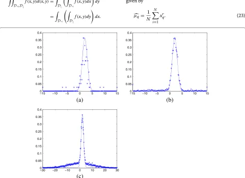
It is well known that the overall performance of a his-togram depends on the number of samples as well as the theoretical PDF. Performances can deteriorate if the num-ber of samples is not large enough. On the other hand, if

realization can be repeated many times, then an accurate estimation of the PDF can be obtained as the average of all obtained histograms (in Figure 13b, the average is done using ten iterations). For a large number of samples, the histogram performs quite well (see Figure 13c).

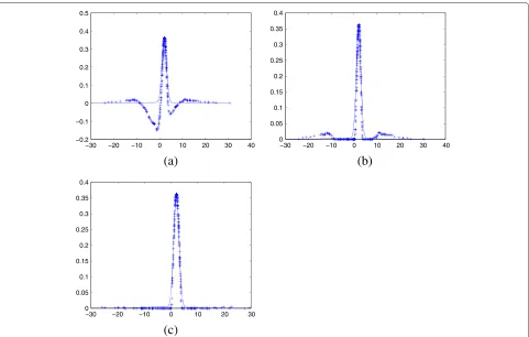
Our simulations show that the Hermite basis set estima-tor suffers from two major inconveniences:

1. It depends on the value ofks,

2. It can generate a negative function, see Figure 14.

The smooth kernel estimator proposed in [46] seems to overcome the previous two mentioned drawbacks (see Figure 15).

8 Conclusions

In this manuscript, a transition indicator for non-stationary signals is presented. The new indicator is based on HOS of quasi non-stationary variables (the random variables are considered stationary by parts). To estimate the HOS, unbiased adaptive exponential estimators are presented.

0 0.5 1 1.5 2 2.5 3 3.5

x 104 _{x 10}4

1.5 2 2.5 3 3.5 4 4.5 5 5.5

Adaptive Variance Filtered by Classification

0 0.5 1 1.5 2 2.5 3 3.5

−40 −35 −30 −25 −20 −15 −10 −5 0

Adaptive Cumulant Filtered by Classification

0 0.5 1 1.5 2 2.5 3 3.5 x 104 −30

−20 −10 0 10 20 30

Derivative of Filtered adaptive Cumulant

Figure 9Derivative of filtered cumulant adaptive estimator.

To reduce the noise level of the HOS estimators, we used a cascade filtering procedure based on Savitzky-Golay fil-ters and a truncation of its Walsh Hadamard transform. Then rectangular signals representing the theoretical val-ues of HOS are obtained by using clustering algorithm using the maxima of kernel PDF estimator and minimiz-ing Euclidean distances.

Simulation studies show that the obtained rectangu-lar signals can suffer from local narrow spurious error windows which can be eliminated using a continuity assumption 1.2 in Appendix 1 and a continuity clean-ing procedure called continuity process. In addition to these local narrow spurious error windows, estimated sig-nals suffer another artifact called the two-step transition problem. After solving this problem using assumption 1.2

0 0.5 1 1.5 2 2.5 3 3.5

x 104 −30

−20 −10 0 10 20 30

Output of IntCont using the continuity process

Figure 10Indicator of non-stationary transition with continuity process.

0 0.5 1 1.5 2 2.5 3 3.5

x 104 −40

−30 −20 −10 0 10 20 30 40

Output of IntCont using continuity and transition processes

Figure 11Indicator of non-stationary transition with continuity and two-step transition processes.

in Appendix 1 and a continuity procedure, an accurate transition indicator of non-stationary signals is achieved. Simulation studies corroborate the performance of our proposed algorithm and the accuracy of our non-stationary transition indicator.

Finally, a survey of major PDF estimators is done. A comparative study is also presented and discussed. The advantages and drawbacks of major methods are high-lighted and a theoretical study is provided. Simulation results show a slight advantage of smooth kernel estima-tor methods. It is worth mentioning that the histogram with a large number of samples is still one of the simplest and efficient estimators. The case of non-stationary pro-cess was considered and a PDF estimation approach was discussed.

Endnotes

a_{However, the processing time is not standardized. In}

fact, different authors claim that the parameters of the channel should remain constant during one frame duration, few hundred symbols, or during the convergence time of their adaptive algorithms.

b_{The fact that the channel is considered as a real}

channel is not limiting our approach, as a complex Gaussian channel could be represented by its modulus as a Rayleigh channel.

c_{The original formula shows the relationship among}

the cumulant ofrstochastic signalsXi(i=1,. . .,r) and

their moments of orderp,p≤r:

Cum[X1,. . .,Xr]=

(−1)k−1(k−1)!

×E

⎡ ⎣

i∈v2 Xi

⎤ ⎦E

⎡ ⎣

j∈v2 Xj

⎤ ⎦. . .E

⎡ ⎣

k∈vp Xk

⎤ ⎦,

Stationary − parts Estimators

HOS

Walsh−Hadamard Smothing Filters N Samples of

Non−Stationary RV

Savitzky−Golay &

PDF Kernel Esimator To find the number & The cluster centers

Nearst−Neighbor Clustering Algorithm

Derivative Filter Digital

Continuity Process

Number & Positions of

Figure 12Synoptic of our algorithm.

where the addition operation is over all the set ofvi(1≤ i≤p≤r) andviconstitutes a partition of{1,. . .,r}, [40].

d_{In many applications, the stochastic signalXis a}

zero-mean signal. This assumption is not a major one and it has been used in many studies (please see [58] and the cited references therein). In fact, by considering this assumption, the mathematical notations can be

simplified. However, all the proposed steps can be straightforwardly derived in the case of a non-zero mean transmission channel. Besides that, the mean can be estimated and canceled out from the other equations.

e_{Further details are given in Appendix 1.}

f_{According to Fubini’s theorem [61], a double integral}

defined over two measure spacesD_a,Dbof a measurable

functionf(x,y)can be computed using iterated integrals:

D,D f(x,y)d(x,y)=

D Df(x,y)dx

dy

=

D

D f(x,y)dy

dx.

g_{A functionf(x)is called Borel’s function if∀y∈}A_is

an open set, the inverse off(x), andx=f−1_{(y)is an}

element of a Borel’s set, i.e., Lebesgue measurable set [62].

h_{Wavelets are basis functions which have quite}

interesting properties such as their localization in space and frequency [24].

Appendix 1: high-order statistics estimators In this section, HOS estimators are developed. Generally, HOS estimators can be divided into main families: the arithmetic and the exponential estimators.

1.1 Arithmetic estimators

LetXto be a zero-mean stochastic ergodic signal where

xiis an event (or a signal sample) ofX(1<i<N). In this

case, the arithmetic estimator of theqth-order moment is given by

μq=

1

N N

i=1

xr_q. (23)

−15 −10 −5 0 5 10 15

0 0.05 0.1 0.15 0.2 0.25 0.3 0.35 0.4

−150 −10 −5 0 5 10 15

0.05 0.1 0.15 0.2 0.25 0.3 0.35 0.4

(a) (b)

−30 −20 −10 0 10 20 30

0 0.05 0.1 0.15 0.2 0.25 0.3 0.35 0.4

(c)

−30 −20 −10 0 10 20 30 40 −0.2

−0.1 0 0.1 0.2 0.3 0.4 0.5

−30 −20 −10 0 10 20 30 40

0 0.05 0.1 0.15 0.2 0.25 0.3 0.35 0.4

(a)

(b)

−30 −20 −10 0 10 20 30

0 0.05 0.1 0.15 0.2 0.25 0.3 0.35 0.4

(c)

Figure 14PDF estimators using Hermite’s polynomial functions with various values ofKs.Theoretical PDF are in continuous curves.(a)

Ks=4.5 without correction.(b)Ks=4.5 with correction.(c)Ks=7.5 without correction.

This estimator assumes that the signalX is stationary overNsamples. This estimator is a non-biased estimator (i.e.,E(μq)=μq) and its variance is given by

Var(μ_q)= μ2q−μ

2 q

N .

Clearly, it is a consistent estimator; hence for stationary signals, its variance decreases with an increased num-ber of samples. An arithmetic estimator of theqth-order cumulant can be developed from Equation 8:

Cum_q(X)=(−1)k−1(k−1)!μ_v1μv2. . . μvp. (24) It is proved [59,60] that the estimator in (24) is a biased consistent estimator where the estimation error decreases proportional to_N1:

ECum_q(X) = q p=1

(−1)p Np−1(p−1)

× ⎛ ⎜ ⎜ ⎜ ⎜ ⎜ ⎝

μq +(N−1)μ_v1μv1

.. .

+(N−1)p−1_μ

v1· · ·μvp

⎞ ⎟ ⎟ ⎟ ⎟ ⎟ ⎠

.

A non-biased cumulant estimator can be deduced from the last equation:

Cum_q(X)= q

p=1

cp(−1)p(p−1)μv1μv2. . . μvp, (25)

−300 −20 −10 0 10 20 30

0.05 0.1 0.15 0.2 0.25 0.3 0.35 0.4

where the parameterscpdepend on the partitions of the

indicesvi. These parameters can be estimated as the

solu-tion ofqlinear equations. Let us consider the fourth-order cumulant:

Cum4(X)=aμ4−4bμ1μ3−3cμ22+12dμ12μ2−6eμ14.

(26)

In order to make the last estimator unbiased, one should solve a linear system of equations obtained by compar-ing term-to-term the expectation of Equation 26 and the theoretical value given by (9)

a= _(NN3₋+₁₎₍N_N2−₋24₂₎₍N_N+₋24₃₎ b= _2(NN(2₋₁₎₍N2_N−₋10₂₎₍N+_N9)₋₃₎

c= _(N−N₁₎₍(N_N2−₋N₂₎₍−_N6)₋₃₎ d= _2(N−N₁₎₍2(2_NN₋−₂₎₍5)_N−3)

e= _(N−1)(NN₋3_2)(N−3)

(27)

For zero-mean signals, we can easily prove that

E(Cum4(X)) = μ4−

This means that the following estimator is an unbiased estimator for the fourth-order cumulant of a zero-mean stationary signalX:

For real-time applications, the estimators should be adap-tive ones. The estimator (23) is not an adapadap-tive one, but it is easy to derive an adaptive version:

thekth iteration.

1.2 Exponential estimators

Exponential estimators are defined as

where 0 < λ_q < 1 represents a forgotting factor. This estimator can be calculated easily in an adaptive way:

but it is asymptotically non-biased. The main interest in

such estimator resides on the fact that it can give bet-ter estimation for the moments of non-stationary signals. Thus, the closestλto 1, the more past samples are taking into account. A non-biased exponential estimator can be written as

Estimator (32) can be also modified to an adaptive version:

An adaptive non-biased estimator of the cumulants could be derived using (22) and (33). To simplify our discussion, the fourth-order cumulant unbiased estimator for zero-mean signals could be developed as

Cum_q(X){k} = Cum_q(X){k−1} +(1−γ )Hk ×Cumq(X){k−1}

whereγ is a forgetting factor and

Hk

1.3 Adaptive unbiased estimators of the fourth-order cumulants

A non-biased estimator of fourth-order cross-cumulants can be obtained from the definition of the cross-cumulants [68]. In fact let us considerK22an estimator of

Cum22(X,Y)defined as

a non-biased and consistent estimator. When samplesxi

andyiare independent, one can use similar estimators to

these proposed in [69,70]. In the following, we assume that the samples are independent and identically distributed (iid) over time but spatially correlated. In this case, one can prove thatK22 become a non-biased and consistent

when a = N_N+₋2₁ andb = c = _NN₋₁. Similarly, one can

To obtain these estimators, signals are assumed sta-tionary. The last assumption cannot be satisfied in our application. Therefore, some modifications should be considered. LetC13(N) =K13(X,Y)be the adaptive

esti-can be written as

N(N−1)C13(N)=(N+2)AN−3BN. (36)

Hence, we can prove that

N(N+1)CN+1=(N+3)AN +xN+1y3_N+1

Finally, the last equation can be modified to

CN = N− equations, we can derive the final form of our adaptive fourth-order cumulant estimator:

Appendix 2: Hermite’s polynomial functions According to [71], Hermite polynomials are real orthog-onal polynomials with respect to the weight function

w(x) = e−x2. The nth-order Hermite polynomial is

Two hermite polynomials of ordersnandmsatisfy the following properties:

m is Kronecker’s symbol. It is worth mentioning

that the above recurrence equation is widely used in prac-tice to estimate the Hermite polynomials. In fact,H0(x)=

1,H1(x) = 2xso H2(x) = 4x2−2 and so on. In order

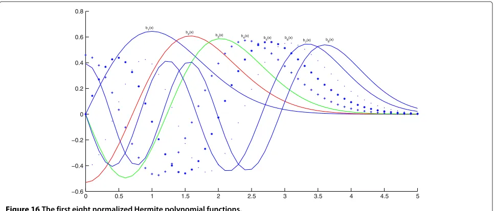
to use Hermite’s basis set, one should define the following two functions:

nomial of the ith order. Figure 16 shows the first eight normalized Hermite polynomial functions, i.e.,bi(x)when ks=1.

Appendix 3: continuity process algorithm

%%%%%%%%%%%%%%%%%%%%%%%%%%%%%%%%%%%%%%%%%%%% % DYcum = IntCont(Ycum,threscon)

%Parameters:

% 1- DYcum indicates the discontinuity of

square functions

% 2- Ycum is sum of noisy square functions

% 3- threscon is the threshold continuity

%Notes:

%%%%%%%%%%%%%%%%%%%%%%%%%%%%%%%%%%%%%%%%%%%% %Author: A. Mansour

%Comments:

%Keywords: Cleaning a noisy square

% indication function % For any comment or bug report, please send

% an e-mail to [email protected]

%%%%%%%%%%%%%%%%%%%%%%%%%%%%%%%%%%%%%%%%%%%% function DYcum = IntCont(Ycum,threscon) DYcum = diff(Ycum);

0 0.5 1 1.5 2 2.5 3 3.5 4 4.5 5 −0.6

−0.4 −0.2 0 0.2 0.4 0.6 0.8

Figure 16The first eight normalized Hermite polynomial functions.

VYcum = DYcum(ndy); % non zero values of DYcum

Dndy = diff(ndy); % intervals of change SInt = find(Dndy < threscon); %indices of

small intervals for i = 1 : length(SInt)

if((VYcum(SInt(i))+VYcum(SInt(i)+1))==0) %error estimated windows create two diracs % of same values but different signs

DYcum(ndy(SInt(i))) = 0; %if an error windows is found then the % change in derivative should be eliminated

DYcum(ndy(SInt(i)+1)) = 0; VYcum(SInt(i)) = 0;

VYcum(SInt(i)+1) = 0; end

end

figure;plot(DYcum);

title(‘Output of IntCont using the continuity process’);

%In some cases, the transition between two %valid states of the Ycum shows two steps. %This case could creates two diracs of the %same sign and close to each other. The %following code is to eliminate this case. ndy = find(DYcum ~= 0);%the indices of non

zero value of the modified DYcum VYcum = DYcum(ndy); % non zero values of

modified DYcum

Dndy = diff(ndy); % intervals of change SInt = find(Dndy < threscon); %indices of

small intervals for i=1:length(SInt)

if((VYcum(SInt(i))* VYcum(SInt(i)+1))>0) %transition error estimated windows create %two diracs of different values but same %signs

CorrectDirac = DYcum(ndy(SInt(i))) + DYcum(ndy(SInt(i)+1));

midledirac = floor((ndy(SInt(i)) + ndy(SInt(i)+1) )/2);

%an integer index in the middle of %the transitions

DYcum( midledirac) = CorrectDirac;

DYcum(ndy(SInt(i))) = 0;

%if an error windows is found then %the change in derivative should be %eliminated

DYcum(ndy(SInt(i)+1)) = 0; VYcum(SInt(i)) = 0;

VYcum(SInt(i)+1) = 0; end

end

figure;plot(DYcum);

title(‘Output of IntCont using continuity and transition processes’);

Appendix 4

The PDF of a moderate sum of two uncorrelated RVs

Let us consider two independent RVsXi,i=1, 2. It is easy

to prove that the proposed random sum can be written as follows:

X=

M

i=1

where,M ∈ 1, 2 is a modified Bernoulli RV, and ais a Bernouilli RV with Pr(a=1)=1−Pr(a=0)=. In this case, one can write:

FX(x) = Pr(X1+aX2≤x)

= Pr(a=0)Pr(X1+aX2≤x|a=0)+Pr(a=1) ×Pr(X1+aX2≤x|a=1)

= (1−)Pr(X1≤x)+Pr(X1+X2≤x) = (1−)FX1(x)+FX1+X2(x).

Using the previous equation, one can deduce [53] that

fX(x)= dF_dxX(x) =(1−)fX1(x)+fX1(x)∗fX2(x),

where * represents the convolution product. If X1

and X2 are two uncorrelated mutually Gaussian RVs,

then Z = X1 + X2 is another normal RV with

, which proves the proposed

statement.

The mean of the new variableXis given by

m=E{X} =m1+m2.

Using the definition of the variance and the properties of a Bernouilli RV, the second moment of the new variable

Xbecomes

In this case the variance ofXcould be obtained as follows:

σ2_=σ2

1+σ22+2(1−)m22.

Competing interests

The authors declare that they have no competing interests.

Authors’ information

AM received his M.Sc. and Ph.D. degrees in Signal, Image and Speech Processing from the ‘Institut National Polytechnique de Grenoble - INPG’ (Grenoble, France) on July 1993 and January 1997, respectively, and his HDR degree (Habilitation a Diriger des Recherches; in the French system, this is the highest of the higher degrees) on November 2006 from the Universite de Bretagne Occidentale - UBO (Brest, France). His research interests are in the areas of blind separation of sources, high-order statistics, signal processing, passive acoustics, cognitive radio, robotics, and telecommunication. From January 1997 to July 1997, he held a post-doc position at Lab. de Traitement d’Images et Reconnaissance de Forme, France. From August 1997 to September 2001, he was a research scientist at the Bio-Mimetic Control Research Center (BMC) in Riken, Nagoya, Japan. From October 2001 to January 2008, he was holding a teacher-researcher position at the Ecole Nationale Supérieure des Ingénieurs des Etudes et Techniques d’Armement (ENSIETA) in Brest, France. From February 2008 to August 2010, he was a senior lecturer at

the ECE Department of Curtin University, Perth, Australia. During January 2009, he held an invited professor position at the Universite du Littoral Cote d’Opale in Calais, France. From September 2010 till June 2012, he was a professor at University of Tabuk, Kingdom of Saudi Arabia. He also served as theelectrical department headat the University of Tabuk. Since September 2012, he has been a professor at Ecole Nationale Supérieure de Techniques Avancées Bretagne (ENSTA Bretagne) in Brest, France. He is the author and the co-author of three books. He is the first author of several papers published in

international journals. He is also the first author of many papers published in the proceedings of various international conferences. Finally, he was elected to the grade of IEEE Senior Member in February 2006. He has been a member of Technical Program Committees (TPC) and he was a chair, co-chair, and a scientific committee member in various international conferences. He is an active reviewer for a variety of international journals. He was a lead guest editor ofEURASIP Journal on Advances in Signal Processing.

RM (S’00-M’08-SM’13) holds a Ph.D. in Electrical Engineering from Jacobs University in Bremen, Germany and several years of post-doctoral wireless communication and optical wireless communication research experience in Germany. In October 2010, he joined University of Tabuk in Saudi Arabia where he is now an assistant professor and the director of research excellence unit. His main research interests are in spatial modulation, MIMO cooperative wireless communication techniques, and optical wireless communication. His publications received more than 800 citations since 2007. He has published more than 50 publications in top-tier journals and conferences, and he holds seven granted patents. He also serves as on the TPC for academic conferences and is a regular reviewer for most of IEEE/OSA Communication Society’s journals and IEEE/OSA Photonics Society’s journals.

HMA received his M.S. and Ph.D. degrees in Electrical Engineering from the University of Washington (UW), Seattle, WA, USA. He is a professional engineer registered in the State of Washington and a senior member of the Institute of the IEEE. He has taught graduate and undergraduate courses in Electrical Engineering at a number of universities in the USA and abroad. He served at many academic ranks including Endowed Chair Professor and Vice President and Provost. He was the winner of the Boeing Supplier Excellence Award. He was also the winner of the IEEE Professor of the Year Award, UW Branch. He is listed as inventor in a major patent assigned to the Boeing Company. His research work is referred to in many patents including patents assigned to ABB, Switzerland, and EPRI, USA. Currently, he is a professor and director of the Sensor Networks and Cellular Systems (SNCS) Research Center, University of Tabuk, Tabuk, Saudi Arabia. He authored many papers in IEEE and other journals and conferences. His research interests include modeling and simulation of large scale networks, sensors and sensor networks, scientific visualization, and control and energy systems.

Acknowledgements

The authors gratefully acknowledge the support for this work by SNCS Research Center at the University of Tabuk under the grant from the Saudi Ministry of Higher Education.

Author details

1_{LAb STIC - ENSTA Bretagne, 2 Rue François Verny, Brest 29200, France.}2_SNCS

Research Center, University of Tabuk, P.O. Box 741, Tabuk 71491, Kingdom of Saudi Arabia.

Received: 1 July 2013 Accepted: 7 February 2014 Published: 20 February 2014

References

1. J Proakis, M Salehi,Digital Communications(McGraw-Hill, New York, 2007) 2. V Tarokh, H Jafarkhani, AR Calderbank, Space-time codes high data rate

wireless communication: performance crirterion and construction. IEEE Trans. Inf. Theory.44(2), 744 (1998)

3. I Bradaric, AP Petropulu, K Diamantaras, On blind identification of FIR-MIMO systems with cyclostationary inputs using second order statistics. IEEE Trans. Signal Process.51(2), 434 (2003)

4. JA Srar, KS Chung, A Mansour, Adaptive array beamforming using a combined LMS-LMS algorithm. IEEE Trans. Antennas Propagation. 58, 3545 (2010)

6. M Abaza, R Mesleh, A Mansour, A Alfalou, MIMO techniques for high data rate free space optical communication system in log-normal channel, inInternational Conference on Technological Advances in Electrical, Electronics and Computer Engineering(TAEECE, Konya, 9–11 May 2013), pp. 161–166

7. M Simon, MS Alouini,Digital Communication over Fading Channels: a Unified Approach to Performance Analysis(Wiley, New York, 2000) 8. S Haykin, M Moher,Communication Systems(Wiley, New York, 2009) 9. M Abaza, R Mesleh, A Mansour, HA Aggoune, Diversity techniques for FSO

communication system in correlated log-normal channels. Opt. Eng. 53(1) (2014). 10.1117/1.OE.53.1.016102

10. VP Skitovic, Linear forms of independent random variables and the normal distribution law. Izvestiya Akademii Nauk SSSR. Seriya Matematiceskaya.18(185) (1954). In Russian

11. M Kendall, A Stuart,The Advanced Theory of Statistics: Distribution Theory (Charles Griffin & Company Limited, London, 1961)

12. CL Nikias, M Shao,Signal Processing withα-Stable Distribution and Applications(Wiley, New York, 1995)

13. J Sijbers, J Den Dekker, P Scheunders, D Van Dyck, Maximum-likelihood estimation of Rician distribution parameters. IEEE Trans. Med. Imaging. 17(3), 357 (1998)

14. GK Karagiannidis, DA Zogas, SA Kotsopoulos, On the multivariate Nakagami-m distribution with exponential correlation. IEEE Trans. Commun.51(8), 1240 (2003)

15. MD Yacoub, G Fraidenraich, JCS Santos Filho, Nakagami-m phase-envelope joint distribution. Electron. Lett.41(5) (2005). doi:10.1049/el:20057014

16. MD Yacoub, G Fraidenraich, HB Tercius, FC Martins, The symmetrical on theη−κdistribution: a general fading distribution. IEEE Trans. Broadcasting.51, 504 (2005)

17. G Fraidernraich, M Daoud Yacoub, Theα−η−μandα−k−μfading distributions, inIEEE 9th International Symposium on Spread Spectrum Techniques and Applications(Manaus, 28–31 August 2006), pp. 255–263 18. S Nadarajah, S Kotz, On theη−κdistribution. IEEE Trans. Broadcasting.

52(3), 411 (2006)

19. MD Yacoub, Theα−ηdistribution: a physical fading model for the Stacy distribution. IEEE Trans. Vehicular Technol.56(1), 27 (2007)

20. SL Cotton, WG Scanlon, J Guy, The_k−μdistribution: applied to the analysis of fading in body to body communication channels for fire and rescue personnel. IEEE Antennas Wireless Propagation Lett.7, 66 (2008) 21. MD Yacoub, Nakagami-m phase-envelope joint distribution: an improved

model, inMicrowave and Optoelectronics Conference, IMOC’2009, (Belem, 3–9 November 2009), pp. 335–339

22. DD Cox, A penalty method for nonparametric estimation of the logarithmic derivative of a density function. Ann. Instit. Stat. Math.37, 271 (1985)

23. J Vidal, A Bonafonte, AR Fonollosa, NF De Losada, Parametric modeling of PDF using a convolution of one-sided exponentials: application to HMM, inEuropean Signal Processing Conference,ed. by M Holt, C Cowan, P Grant, W Sandham, European Signal Processing Conference(Elsevier, Edinburgh, 1994), pp. 54–57

24. M Vannucci, Nonparametric density estimation using wavelets. Discussion Paper, Duke University, 1998

25. A Archambeau, M Verleysen, Fully nonparametric probability density function estimation with finite gausssian mixture models, in5th International Conference on Advances in Pattern Recognition Calcultta, ICAPR’2003, (Allied, New Delhi, Calcultta, 2003), pp. 81–84

26. R Boscolo, H Pan, VP Roychowdhury. IEEE Trans. Neural Netw.15(1), 55 (2004)

27. F Roueff, T Rydén, Nonparametric estimation of mixing densities for discrete distributions. Ann. Stat.33(5), 2066 (2005)

28. S Alamouti, A simple transmit diversity technique for wireless communication. IEEE J. Selected Areas Commun.16(8), 1451 (1998) 29. EG Larsson, P Stoica,Space-time Block Coding for Wireless Communications

(The Press Syndicate of the University of Cambridge, Cambridge, 2003) 30. V Choqueuse, A Mansour, G Burel, L Collin, K Yao, Blind channel

estimation for STBC systems using higher-order statistics. IEEE Trans. Wireless Commun.10, 495 (2011)

31. A Mansour, C Jutten, N Ohnishi, Kurtosis: definition and properties, in International Conference on Multisource-Multisensor Information Fusion, ed. by HR Arabnia, DD Zhu, (Las Vegas, 6–9 July 1998), pp. 40–46

32. A Mansour, C Jutten, What should we say about the kurtosis. IEEE Signal Process. Lett.6(12), 321 (1999)

33. JM Mendel, Tutorial on higher-order statistics (Spectra) in signal processing and system theory: theoretical results and some applications. IEEE Proc.79, 277 (1991)

34. A Cichocki, SI Amari,Adaptive Blind Signal and Image Processing: Learning Algorithms and Applications(Wiley, New York, 2002)

35. JF Cardoso, Source separation using higher order moments, in Proceedings of International Conference on Speech and Signal Processing 1989, ICASSP 1989, (Glasgow, 22–25 May 1989), pp. 2109–2212 36. P Comon, Independent component analysis, a new concept Signal

Process.36(3), 287 (1994)

37. A Mansour, C Jutten, A direct solution for blind separation of sources. IEEE Trans. Signal Process.44(3), 746 (1996)

38. A Hyvärinen, J Karhunen, E Oja,Independent Component Analysis (Wiley, New York, 2001)

39. A Mansour, A Kardec Barros, N Ohnishi, Blind separation of sources: methods, assumptions and applications. IEICE Trans. Fundamentals Electron. Commun. Comput. Sci.E83-A(8), 1498 (2000)

40. A Papoulis,Probability, Random Variables, and Stochastic Processes (McGraw-Hill, New York, 1991)

41. M Rosenblatt, Remarks on some nonparametric estimates of a density function. Ann. Math. Stat.27(3), 832 (1956)

42. E Parzen, On the estimation of a probability density function and mode. Ann. Math. Stat.33(3), 1065 (1962)

43. LN Bowers, Expansion of probability density functions as a sum of gamma densities with applications in risk theory. Trans. Soc. Actuaries.

18 PT 1(52), 125 (1966)

44. HV Khuong, HY Kong, General expression for pdf of a sum of independent exponential random variables. IEEE Commun. Lett.10(3), 159 (2006) 45. CH Reinsch, Smoothing by spline functions. Numer. Math.10, 177

(1967)

46. AW Bowman, A Azzalini,Applied Smoothing Techniques for Data Analysis (Oxford University, New York, 1997)

47. SC Schwartz, Estimation of probability density by an orthogonal series. Ann. Math. Stat.38(3), 1261 (1967)

48. M Vannucci, On the application of wavelets in statistics. Ph.D. thesis, Dipartimento di Statistica, University of Florence, 1996

49. J Engel, Density estimation with, Haar series. Stat. Probability Lett.9, 111 (1990)

50. S Kay, Model-based probability density function estimation. IEEE Signal Process. Lett.5(12), 318 (2001)

51. J Xie, Z Wang, Probability density function estimation based on windowed Fourier transform of characteristic function, inProceedings of the 2nd International Congress on Image and Signal Processing, (Tianjin, 17–19 October 2009)

52. RM Howard, PDF estimation via characteristic function and an orthonormal basis set, inProceedings of the 14th WSEAS International Conference on Systems, (Corfu, 23–25 July 2010), pp. 100–105

53. A Mansour,Probabilités et statistiques pour les ingénieurs: cours, exercices et programmation(Hermes Science, Paris, 2007)

54. R Mesleh, H Haas, S Sinanovic, CW Ahn, S Yun, Spatial modulation. IEEE Trans. Vehicule Technol.57(4), 2228 (2008)

55. Z Wang, GB Giannakis, A simple general parameterization quantifying performance in fading channels. IEEE Trans. Commun.51(8), 1389 (2003) 56. P McCullagh,Tensor Methods in Statistics(Chapman and Hall, London,

1987)

57. AN Shiryayev,Probability(Springer, London, 1984)

58. MH Vu, Exploiting transmit channel side information in MIMO wireless systems. Ph.D. thesis, Stanford University, 2006

59. S Kotz, NL Johnson,Encyclopedia of Statistical Sciences(University of Amesterdam, Amesterdam, 1993)

60. JL Lacoume, PO Amblard, P Comon,Statistiques d’ordre supérieur pour le traitement du signal(Mason, Paris, 1997)

61. J Bass,Cours de Mathématiques: Tome 1, Fasicule 2(Masson, Paris, New York, Barcelone et Milan, 1977)

62. J Bass,Cours de Mathématiques: Tome 2(Masson, Paris, New York, Barcelone et Milan, 1977)

64. A Savitzky, MJE Golay, Soothing and differentiation of data by simplified least squares procedures. Anal. Chem.36, 1627–1639 (1994)

65. SJ Orfanidis,Introduction to Signal Processing(Prentice-Hall, New Jersey, 1995)

66. RW Schafer, What is a Savitzky-Golay filter? IEEE Signal Process. Mag, 111–117 (2011)

67. K Beauchamp,Applications of Walsh and Related Functions (Academic, New York, 1984)

68. M Kendall, A Stuart,The Advanced Theory of Statistics: Design and Analysis, and Time-series(Charles Griffin & Company Limited, London, 1961) 69. A Mansour, A Kardec Barros, N Ohnishi, Comparison among three

estimators for high order statistics, inFifth International Conference on Neural Information Processing (ICONIP’98), ed. by S Usui, T Omori, (Kitakyushu, 21–23 October 1998), pp. 899–902

70. A Martin, A Mansour, Comparative study of high order statistics estimators, inInternational Conference on Software, Telecommunications and Computer Networks, (Split, Dubrovnik, Venice, 10–13 October 2004), pp. 511–515 71. A Bouvier, M George, F Le Lionnais,Dictionnaire des mathématiques

(Presses Universitaires De France, Paris, 1993)

doi:10.1186/1687-6180-2014-21

Cite this article as:Mansouret al.:Blind estimation of statistical properties of non-stationary random variables.EURASIP Journal on Advances in Signal Processing20142014:21.

Submit your manuscript to a

journal and benefi t from:

7Convenient online submission

7 Rigorous peer review

7Immediate publication on acceptance

7 Open access: articles freely available online

7High visibility within the fi eld

7 Retaining the copyright to your article