R E S E A R C H
Open Access
Self-adaptive algorithm for segmenting skin
regions
Michal Kawulok
*, Jolanta Kawulok, Jakub Nalepa and Bogdan Smolka
Abstract
In this paper, we introduce a new self-adaptive algorithm for segmenting human skin regions in color images. Skin detection and segmentation is an active research topic, and many solutions have been proposed so far, especially concerning skin tone modeling in various color spaces. Such models are used for pixel-based classification, but its accuracy is limited due to high variance and low specificity of human skin color. In many works, skin model adaptation and spatial analysis were reported to improve the final segmentation outcome; however, little attention has been paid so far to the possibilities of combining these two improvement directions. Our contribution lies in learning a local skin color model on the fly, which is subsequently applied to the image to determine the seeds for the spatial analysis. Furthermore, we also take advantage of textural features for computing local propagation costs that are used in the distance transform. The results of an extensive experimental study confirmed that the new method is highly competitive, especially for extracting the hand regions in color images.
Keywords: Skin detection; Skin segmentation; Adaptive color model; Spatial analysis
1 Introduction
Detection and segmentation of human skin regions [1,2] in color images is an active research topic, which receives considerable attention from image and signal processing community. Skin detection consists in taking a binary decision whether an image, its region, or a particular pixel presents the human skin. In case of the positive answer, skin segmentation is applied to determine the exact boundaries of the detected skin regions. Applica-tions of skin detection and segmentation are of a wide range and significance, and they include gesture recog-nition for human-computer interaction [3], objectionable content filtering [4], content-based image retrieval [5], medical imaging [6,7], and image coding [8].
1.1 Overview of skin detection and segmentation techniques
The existing methods are based on the premise that the skin color can be effectively modeled in various color spaces, which allows segmenting the skin regions in color images. Using skin color models, every pixel may be classified to the skin or non-skin class based on its
*Correspondence: [email protected]
Faculty of Automatic Control, Electronics and Computer Science, Silesian University of Technology, Akademicka 16, 44-100 Gliwice, Poland
position in the color space, independently from its neigh-bors. Alternatively, the probability that each pixel presents the skin can be determined, which transforms a color image into askin probability map(PS). The map may be binarized using a certain acceptance threshold in order to extract the skin regions. This problem has been widely studied, and a large number of skin color models were introduced over the years. The main difference between them lies in their learning and generalization capabilities, but given a sufficiently large training set, their effective-ness is similar, and it is limited due to high variance and low specificity of human skin color [2]. Basically, skin and non-skin pixels overlap in color spaces; hence, they can-not be separated relying exclusively on their color. The pixel-wise classification may be improved by incorporat-ing information extracted from the texture, as well as by spatial analysis of the pixels that have high skin probability. Also, global skin color models may be adapted to a par-ticular scene or an individual who appears in the image, which improves the classification accuracy, providing that the adaptation is correct.
1.2 Contribution
In the work reported here, we introduce a new method that consists in combining three important elements,
namely, (i) skin color model adaptation, (ii) spatial anal-ysis, and (iii) exploitation of the textural features. First, a skin probability map is obtained from the input image using a global model. The map is processed to extract skin samples, used to create a local skin color model. Subse-quently, the local model is applied to locate the seeds for spatial analysis, which determines the final boundaries of the skin regions. We perform the spatial analysis using the discriminative skin-presence features(DSPF), introduced in our earlier work [9], that rely on textural properties of skin probability maps.
There have been a handful of methods proposed [10,11] that combine model adaptivity with spatial analysis. These techniques require a skin sample for the adaptation, deliv-ered by a face detector, and they do not exploit textural features. Naturally, these methods cannot perform the adaptation when a face is not visible or if a face detector fails.
In the proposed approach, the model is adapted based on analysis of a skin probability map, without using any additional information sources. The reported exper-imental results clearly show that our algorithm achieves better segmentation scores than alternative state-of-the-art methods. Furthermore, the new method significantly increases the detection precision, which is particularly important when a hand region is to be segmented for the hand pose estimation purposes.
1.3 Paper structure
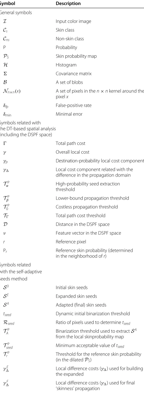
The paper is organized as follows. In Section 2, the exist-ing approaches to skin detection and segmentation are outlined, with particular attention given to the adaptation techniques. Spatial analysis methods used in our study are described in Section 3, and the proposed skin detection algorithm is presented in details in Section 4. Experi-mental validation is reported and discussed in Section 5. Section 6 concludes our study. Furthermore, the symbols used in the paper are explained in Table 1.
2 Related literature
Skin detection and segmentation has been widely studied over the last 20 years, and a lot of advancements emerged so far. A large number of contributions address the prob-lem of skin color modeling in various color spaces, and they are well summarized in a survey published in 2007 by Kakumanu et al. [1].
Skin color can be modeled using a set of rules and thresholds defined in color spaces based on some obser-vations [12-15]. Alternatively, given a representative train-ing set, skin detection rules can be determined ustrain-ing machine learning. Jones and Rehg [16] proposed to train the Bayesian classifier in the RGB space. This requires a training set containing pixels assigned to the skin (Cs) and non-skin (Cns) classes. Color histograms are built for these
Table 1 The symbols used in the paper
Symbol Description
γp Destination-probability local cost component γ Local cost component related with the
difference in the propagation domain
TP
T Total path cost threshold
D Distance in the DSPF space ν Feature vector in the DSPF space
r Reference pixel
Pr Reference skin probability (determined
in the neighborhood ofr)
Symbols related with the self-adaptive seeds method
S0 Initial skin seeds
SE Expanded skin seeds
SA Adapted (final) skin seeds
tseed Dynamic initial binarization threshold Rseed Ratio of pixels used to determinetseed TP
A Binarization threshold used to extractSA
from the local skinprobability map
TP
seed Minimum acceptable value oftseed TP
r Threshold for the reference skin probability
(in the dilatedPS) γE
Local difference costs (γ) used for building the expanded
γF
two classes: P(v|Cs)and P(v|Cns), wherevis the color, and the probability that a given pixel presents the skin (i.e., P(Cs|v)) is determined from the Bayes rule. This is a robust approach, provided that a sufficiently large training set is available. In the majority of cases, it is beneficial to reduce the number of histogram bins per channel to increase the generalization capacity [2,17]. Analysis of color his-tograms has also been applied to solve more general tasks concerning extracting image regions [18].
Greenspan et al. [19] used Gaussian mixture models (GMMs) for learning human skin color in the normalized rgchromaticity space. GMMs offer better generalization capabilities than the Bayesian classifier, and they were later exploited in many approaches to skin color mod-eling [20,21]. In our recent survey [2], we demonstrated that GMMs outperform the Bayesian classifier for small training sets; however, for larger sets, the latter was more accurate.
Among other machine learning techniques applied to skin detection, it is worth to mention artificial neural net-works (ANNs) [22,23], support vector machines [24,25], and random forests [10]. In general, the methods based on machine learning achieve higher classification accuracy than the rule-based approaches.
Skin detection and segmentation plays also an impor-tant role in dermoscopy for skin lesions segmentation and analysis. This is an active research topic of med-ical imaging, and many methods have been developed over time [6]. Segmentation of skin lesions may be performed using a number of techniques, which take advantage of the skin homogeneity in the domain of color, luminance or texture, and they include statisti-cal region merging [26,27], dynamic programming [28], and wavelet-based texture analysis [7]. The segmenta-tion phase is followed by shape analysis to investigate the lesion type [29]. In general, these methods are spe-cialized to deal with the dermoscopy images. It is there-fore assumed that a given image presents human skin with some lesions that should be segmented from the background.
2.1 Adaptive skin color modeling
Accuracy of skin detection using color models is limited due to the overlapping between skin and non-skin pix-els, which may be observed in various color spaces. If the model is created so that it omits the overlapping val-ues, then many skin pixels are classified as background, decreasing the recall. On the other hand, if the model includes these overlapping values, then the number of false-positives (FP) is increased. It is worth noting that the overlap may be reduced, if a skin model is adapted to indi-viduals who appear in a presented scene. Given constant lighting conditions and a limited number of individuals in the image, skin color specificity is definitely higher than in
the general case, and overall, the skin regions can be better separated from the background.
Basically, the existing adaptation methods either require a skin sample, from which the local skin model is learned on the fly, or they use some features extracted from an input image to fit the model. In the latter case, sev-eral approaches exploit ANNs for the adaptation. Lee et al. [4] used a multilayer perceptron to select the most appropriate skin model from a collection of models, each of which was trained earlier for specific lighting condi-tions. ANNs were also used to tune the parameters of the Gaussian intended to model the skin color, given an image histogram [30], as well as to determine an optimal acceptance threshold [31] for each skin probability map obtained using a global model. Sun [32] applied a global skin model to extract skin pixels, whose distribution was subsequently modeled using GMM. Final skin probabil-ity was determined relying on that locally learned GMM combined with the global model. In this way, those pixels preliminarily classified as skin, which do not form clusters in the color space, are reclassified as background.
Skin models can also be effectively adapted given a skin sample, acquired based on tracking skin-like objects in video sequences [33], or relying on face [11,34] or hand [3] detection. For such a skin sample, a local model can be generated using the Bayesian classifier [35,36] or GMMs [37] as they do not require time-consuming train-ing. However, although the local model allows detecting the skin with high precision, the recall is often low. To address this problem, the local model is combined with the global one. The final probability Pf(Cs|v)can be com-puted as a weighted mean of the probabilities obtained using the local Pl(Cs|v)and global Pg(Cs|v)models.
Another approach adopted here consists in using a global skin color locus, which imposes a restriction on the adaptation [37,38]. It is also possible to combine the local and global models by incorporating them into a spatial analysis framework, which is given more attention later in this section.
Alternatively, a skin sample may be used to opti-mize the value of the acceptance thresholds [3,39]. Recently, Yogarajah et al. [40] proposed to use skin sam-ples for adapting the acceptance thresholds in a single-dimensional error signal space (ESS) [14]. ESS is obtained from RGB, and skin color can be modeled here using a single Gaussian.
The Yogarajah’s method consists in analyzing the dis-tribution of the error signal in a facial region to deter-mine the decision thresholds from the obtained Gaussian parameters.
2.2 Textural and spatial analysis
[41] demonstrated that even for perfect adaptation, in most situations, the skin cannot be completely separated from the background in a given color space. The discrimi-native power of skin classifiers may be increased, when the pixels neighborhood is taken into account, for example, exploiting textural features extracted from an input image. Wang et al. [42] proposed to enhance the segmenta-tion in the RGB and YCgCb color spaces by analyzing various textural features, extracted using the gray-level co-occurrence matrix. Moreover, simple textural features were used to boost the performance of a number of skin detection techniques and classifiers, including the ANNs [43], parametric density estimation of skin and non-skin classes [44], GMMs [45], and many more [46-49]. In our earlier work [50], we found it beneficial to extract tex-tural features from skin probability maps rather than from the input images.
Skin detection accuracy may also be increased using the region-growth operations, because skin pixels are usually grouped, whereas the non-skin false-positives are scat-tered in the spatial domain. Here, conventional image segmentation algorithms can be applied, for example, those based on combined Markov random fields [51], or probabilistic bottom-up aggregation [52]. It may be ben-eficial to extract and utilize some textural features, for example, using wavelets [7,53]. Although this is a time-consuming technique, it has been demonstrated that it may be successfully optimized for DSP processors [54]. Overall, a number of specific methods devoted to seg-menting skin regions have been developed. Kruppa et al. [5] proposed to verify the potential skin regions assuming that they should have an elliptical shape. In other works, a threshold hysteresis in skin probability maps was applied to accept those regions, which are connected with the seeds of high skin probability [36,55]. Furthermore, spatial properties of skin regions were analyzed using conditional random fields [56] and cellular automata [49]. Del Solar and Verschae proposed to analyze skin probability maps using controlled diffusion [57]. At first, the diffusion seeds are formed by those pixels, whose skin probability exceeds theseed threshold(TαP). Then, the neighboring pixels are iteratively adjoined to the skin region, if they meet the diffusion process criteria, provided that their skin proba-bility is larger than thelower-bound propagation threshold
(TP
β).
In our earlier research [58], we introduced an energy-based technique for skin blobs analysis. The skin regions are expanded depending on the amount of energy, which is spread over the image, according to the local skin prob-ability. Recently, we proposed to use the distance trans-form (DT) in a combined domain of hue, luminance, and skin probability [59,60]. Furthermore, we elaborated on the importance of seeds detection, from which the skin probability (termed ‘skinness’) is propagated. This method
is exploited in the research reported here, and it is given more attention in Section 3.
2.3 Hybrid methods
There are relatively few methods that combine the afore-mentioned improvement strategies, and the research reported in this paper also falls into this category.
Jiang et al. [61] proposed to take advantage of color, tex-ture, and space analysis. At first, the skin regions are deter-mined based on a skin probability map obtained from color information. Subsequently, the regions are refined to improve the precision, relying on the textural features extracted using the Gabor wavelets. Finally, the regions are grown with the watershed segmentation to exploit the spatial information.
Combining textural features with spatial analysis was also the key contribution of our recent work [9]. We intro-duced the DSPF space, which is exploited to compute the local costs for DT, instead of using the skin probability map as in [59]. As we also use the DSPF domain in our study, this method is given more attention in Section 3.
In our another work [11], we explored how to combine a local skin color model with the global one using spatial analysis. We applied the face-based local model to detect the skin seeds, from which the ‘skinness’ is propagated using DT to adjoin the skin pixels. A similar approach was proposed by Khan et al. [62], where the local model is learned from the facial region. The model is used to obtain the foreground weights for the graph-cut image segmentation, and the background weights are obtained using the global skin color model. A potential drawback of this method lies in using a generic image segmenta-tion algorithm, whose parameters are difficult to tune. Unfortunately, the implementation is not available, and the paper does not include all the details necessary to reproduce the results. The method was validated using thousands of video frames. Although this is a huge data set, the number of scenes and individuals is quite small, as the images were extracted from only 25 videos and the conditions within each single video are uniform. Also, the authors claim to have used 8,991 images for validation, while the entire data set contains 10,764 frames, and it is unclear which images were excluded. Last, but not least, the method is quite slow, as it requires 1.5 s to process a small 100×100 image.
3 Distance transform for spatial analysis
3.1 Propagation seeds
The aim of the seeds extraction is to determine the ini-tial skin regions, from which the ‘skinness’ is propagated. The seeds are considered as skin, and neighboring pix-els are subsequently adjoined to the skin region using DT. In an ideal case, not only should the seeds contain no false-positive pixels but also every ground-truth skin blob (i.e., a region composed of the real skin pixels) should include at least one detected seed inside. Otherwise, such a region would not be adjoined to the skin class during the propagation, increasing the false-negative (FN) rate.
The seeds can be extracted taking advantage of the observation that if the skin probability map is binarized using a high-probability threshold, then the precision is rather high, because usually only true-positive (TP) skin regions contain pixels with very high skin probability val-ues. If the skin probability of an individual pixel is over a high thresholdTP
α, then the pixel is added to the seed. Such an approach was adopted in many spatial analysis methods [36,55,57].
Recently, we proposed to create an adaptive seed based on detected facial regions [11]. Using the geometrical fea-tures extracted from the luminance channel of the input color image, the facial regions are detected. A local skin model is learned using a single multivariate Gaussian, and the model is applied to the input image to obtain a local skin probability map, which is binarized to determine the final seeds. Afterwards, the propagation is carried out using the skin probability map obtained from a global skin color model.
3.2 ‘Skinness’ propagation
In order to propagate the ‘skinness’ from the seeds, the shortest routes from the seed to every pixel are deter-mined at first. This is achieved by minimizingtotal path costsfrom the set of seed pixels to each non-seed pixel in the image. The total path cost for a pixelxis defined as
(x)= l−1
i=0
γ (pi→pi+1), (1)
whereγ is a local propagation cost between two neigh-boring pixels,p0is a pixel that lies at the seed boundary,
pl = x, andl is the total path length. The minimization is performed using the Dijkstra’s algorithm [63]. In addi-tion, the thresholdTβP = 0.3 is used as proposed in [57], which prevents propagating to the regions of very low skin probability. Furthermore, mainly to decrease the execu-tion time, the propagaexecu-tion is terminated if the total path cost exceeds a certain boundary valueT.
The route optimization outcome heavily depends on how the local costsγ are computed. For skin segmenta-tion, we construct the local cost using two major compo-nents, namely the difference in the propagation domain
γand the destination-probability costγp. The local cost from a pixelxtoy, i.e.,γ (x→y)is obtained as the costless propagation threshold (if the skin probability at pixelyexceeds T0P, then the total path cost does not increase when moving from pixelxto y). The difference costγ was originally defined using hue and luminance values:
γ(x,y)=αd· Y(x)−Y(y) + H(x)−H(y) , (4)
whereαd ∈ {1, √
2}is the penalty for propagation in the diagonal direction,Y(·)is the pixel luminance, andH(·)is the hue in the HSV color model, both scaled to the range from 0 to 255.
The total path cost obtained after the optimization is inversely proportional to the ‘skinness’; hence, the final skin probability map is obtained by scaling the costs from 0 (for the maximal cost) to 1 (for a zero cost, i.e., the seed pixels). The pixels not adjoined during the propagation process (i.e., those whose total path costis greater than T) are assigned with zeroes. Finally, the skin regions are extracted using a fixed threshold in the distance domain.
In the research reported in this paper, we consider alternative local difference costs (explained below), which we found effective in various ‘skinness’ propagation scenarios.
1. Restrictive hue-luminance difference cost:
γ(HL)
(x,y)=αd·max Y(x)−Y(y) , H(x)−H(y) . (5)
2. Cost based on a difference in the RGB color space:
γ(RGB)
(x,y)=αd· R(x)−R(y) + G(x)−G(y) + B(x)−B(y) . (6)
3. Skin probability difference cost:
γ(SP)
(x,y)=αd· PS(x)−PS(y) . (7)
3.3 Discriminative skin-presence features domain
The textural features are incorporated into the DSPF space, later exploited to refine the skin probability. In order to obtain the DSPF space, the basic image fea-tures are first extracted from the skin probability map. They consist of the following features: (i) themedianand (ii) minimalvalues, (iii)standard deviation, and (iv) the difference between the maximum and minimum, com-puted in three kernels: 5×5, 9×9, and 13×13 pixels. In addition, the raw skin probability value is appended to this feature vector, as it is the principal source of the discriminating information between skin and non-skin pixels. We considered exploiting more advanced textural descriptors, for example, local binary patterns [64]; how-ever, it has not improved the results. The selected features are aimed at extracting the roughness of the skin probabil-ity map rather than finding a repeatable pattern, and this can effectively be done using these simple statistics. Over-all, every pixel x is transformed into an M-dimensional basic feature vector ux, where M = 13. Using linear
discriminant analysis, the dimensionality of the basic image feature space is reduced tom=2 dimensions in the DSPF space.
Subsequently, a pixel of maximum skin probability is found in the skin probability map eroded using a large (15×15) kernel; it should be larger than the kernels used for extracting basic image features. This pixel is termed thereference pixel r, and the distance betweenrand every pixel in the image is computed in the DSPF space:
D(x)=
m
i=1
ν(x) i −ν(ir)
21/2
, (8)
where νi(x) is the ith dimension of the DSPF vector obtained for the pixel x. This operation converts the input skin probability map into the DSPF skin map, which is normalized and used for computing the destination-probability costγp.
4 Skin segmentation using self-adaptive seeds In this section, we present the details of the proposed approach. Compared with our earlier methods, here, our main contribution lies in introducing a new technique for extracting adaptive seeds, which does not require any skin sample be givena priorifor the adaptation. Instead of exploiting a face detector to acquire the skin sam-ple, we analyze the skin probability map PS obtained from the input color imageI using a global skin color model. At first, our algorithm determines whether the image presents any skin pixels at all, and subsequently, it extracts the skin sample that is used to adapt the skin model and to build the seeds. Furthermore, we elabo-rate on the adaptation scheme we introduced in [11] and apply new metrics to compute local costs for DT [59]. These metrics (Equations 5 to 7) are used for creating the seeds, as well as they are utilized for the final ‘skinness’ propagation.
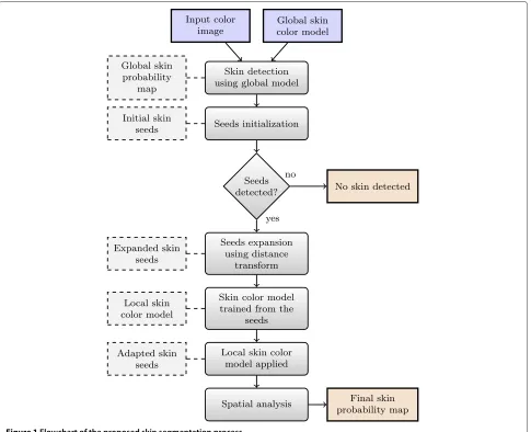
4.1 Algorithm outline
A flowchart of our method is presented in Figure 1, and examples of outcomes obtained at subsequent stages of the processing chain are demonstrated in Figure 2. First of all, an input image (Figure 2(a)) is converted into a skin probability map (Figure 2(b)) using a global skin color model based on the Bayesian classifier (the darker shade indicates higher skin probability). The obtained skin probability map is processed to determine theinitial skin seeds(annotated as red pixels inside the black regions in Figure 2(c)). Here, our goal is to extract a sample of skin pixels with high precision, without including the non-skin pixels. Although it is crucial that the seeds are detected in every ground-truth skin blob, this is not critical at this stage, as the seeds are transferred to other regions later. An important problem here is to avoid finding the initial skin seeds in the images which do not contain human skin at all; otherwise, the algorithm may adapt the skin model
(a)
(b)
(c)
(d)
(e)
(f)
(g)
to some non-skin regions, increasing the false-positive rate. The exact procedure on how the initial seeds are determined is described later in Section 4.2.
Subsequently, the initial seeds are expanded using DT to include more skin pixels (black regions in Figure 2(c)). Again, the primary goal at this stage is to keep the false-positive rate at the smallest pos-sible level; hence, the conditions for adjoining the pixels should be strict. From the expanded seeds, a local skin color model is trained and applied to the image in order to determine the final seeds for the
propagation (black regions in Figure 2(d)). Here, the aim is to find at least a single seed in every ground-truth skin region while keeping the false-positives low. It can be seen from Figure 2(d) (images I to IV) that the adapted seeds appear in the skin regions which were not cov-ered by the initial skin seeds, while they are absent in the background. For image V, the seeds are not trans-ferred to new skin regions, but the adaptation allows the seeds to be better distributed in the regions already cov-ered by the expanded seeds. Also, an interesting case is image VI; here, the adaptation almost does not modify the
(a)
(b)
(c)
(d)
position of the expanded seeds; however, eventually, the initial seeds occur sufficient to propagate the ‘skinness’ over the entire skin area. The details of the seed transfer are given in Section 4.3.
From the final seeds, the ‘skinness’ is propagated over the image to obtain the final skin probability map (Figure 2(e)), which is binarized to extract the skin regions (see Figure 2(f ), where the red tone indicates false-positive pixels, the blue tone false-negatives, and the green one boundaries of the true-positive regions).
In Figure 2(g), we present the segmentation results obtained from the global skin probability maps (from Figure 2(b)). For several images (I to III), the adapta-tion substantially reduced the false-positives (which were caused by the background objects having skin-like color). Both the false-positives and false-negatives were reduced for the images III to V, and in the case of image VI, the false-negative rate was decreased.
4.2 Extracting initial skin seeds
This stage consists in finding initial skin samples, from which the proper seeds for propagation are later created. In our method, this is achieved exclusively based on the analysis of a skin probability map obtained using a global skin color model (we utilize the Bayesian classifier here; however, other skin color models may also be exploited for this purpose). The initial skin seeds are extracted relying on the skin probability histogram and by analyzing the pixels in the spatial domain.
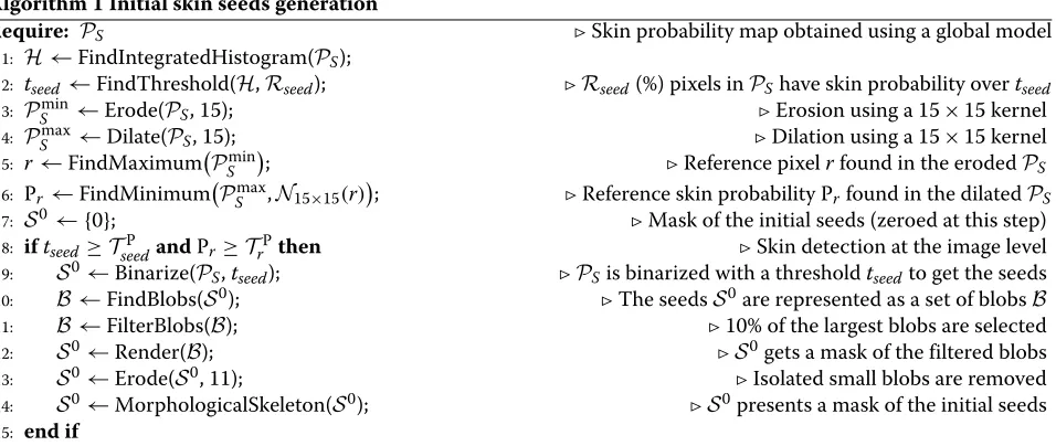
The algorithm for finding the initial seeds is out-lined in Algorithm 1. First, we compute the integrated
histogram H (line 1) of the skin probability map PS
to find the value of a dynamic threshold tseed, which selects Rseed = 5% pixels, whose probability is above tseed (line 2). Afterwards, we determine the reference
pixel rthat indicates the maximum probability value in the eroded skin probability map Pmin
S (line 5).
Subse-quently, we compute the reference skin probability Pr (line 6) as the minimum probability value in the dilated skin probability map PSmax within the 15× 15 neigh-borhood of the reference pixel (N15×15(r)). Basically, if
the reference pixel presents the skin indeed, then the value of the reference skin probability Pr should be high.
Based on the values of Prandtseed, we take the decision (Algorithm 1, line 8) whether an image contains skin pix-els at all (hence, we detect skin at the image level). This is an important step of our algorithm, as false-positive detection would lead to adapting the skin color model to non-skin pixels, significantly decreasing the overall seg-mentation precision. On the other hand, false-negative detection would mean that the entire skin area in the incorrectly classified image is rejected. We apply fairly simple rules here that consist in checking whether the Pr andtseedvalues are above the thresholdsTrP = 0.24 and TP
seed = 0.12, respectively. Efficacy of this technique is discussed later in Section 5.
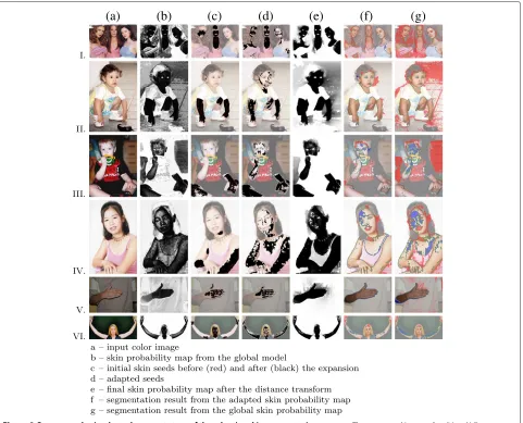
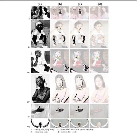
If the image-level skin detection is positive, then the seeds are extracted by binarizing the skin probability map using thetseed threshold (Algorithm 1, line 9). We have observed that the false-positive pixels are scattered in the binarized image, while the true-positive pixels are orga-nized in spatially consistent groups. Following this obser-vation, we use only 10% of the largest blobs (line 11). These blobs are additionally subject to the erosion (line 13) to eliminate the blobs having small area. Finally, the seeds are subject to the morphological skeletonization (line 14), which further reduces the false-positives. The results obtained in subsequent steps of the initial skin seeds extraction are presented in Figure 3.
Algorithm 1 Initial skin seeds generation
Require: PS Skin probability map obtained using a global model
1: H←FindIntegratedHistogram(PS);
2: tseed←FindThreshold(H,Rseed); Rseed(%) pixels inPShave skin probability overtseed
3: PSmin←Erode(PS, 15); Erosion using a 15×15 kernel
; Reference skin probability Prfound in the dilatedPS
7: S0← {0}; Mask of the initial seeds (zeroed at this step)
8: iftseed≥TseedP andPr ≥TrPthen Skin detection at the image level
9: S0←Binarize(PS,tseed); PSis binarized with a thresholdtseedto get the seeds
10: B←FindBlobs(S0); The seedsS0are represented as a set of blobsB
11: B←FilterBlobs(B); 10% of the largest blobs are selected
12: S0←Render(B); S0gets a mask of the filtered blobs
13: S0←Erode(S0, 11); Isolated small blobs are removed
14: S0←MorphologicalSkeleton(S0); S0presents a mask of the initial seeds
4.3 Seed expansion and adaptation
The initial skin seeds are characterized with two gen-eral properties (confirmed experimentally): (i) the seeds indicate skin regions with very high precision (i.e., they contain very few false-positives), and (ii) they are not present in every ground-truth skin blob (see Figure 2(c)). The first property makes the seeds appro-priate to initiate DT in order to determine the bound-aries of those skin regions, in which the seeds appear. However, the second property means that the ‘skinness’ cannot be propagated in the spatial domain to non-covered skin blobs; hence, the color space must be used for transferring the ‘skinness’. This transfer is achieved by creating a local skin color model from the ini-tial skin seeds and applying it to the entire image. After this operation, the seeds are expected to appear in every skin blob, and they are used for the final propagation.
Overall, the skin segmentation algorithm, including the detailed procedure for extracting the final seeds, is given in Algorithm 2. After obtaining the initial seeds, they are expanded using DT (line 3) to include more skin pix-els (this forms theexpanded skin seedsSE). Without the expansion, the model built from the initial seeds would not be sufficiently representative and the seeds would not be correctly transferred in the color space. However, the expansion must be done carefully to avoid including non-skin pixels, which could eventually lead to transferring the seeds also into the background. We investigated various local costs for obtainingSE termedγE; however, in all the cases, we impose the cost boundaryT=3·γE, where
γE
is the average local cost computed within the image. Furthermore, we do not use the costless propagation here
i.e., T0P=0. This limits DT to the very neighborhood of the initial seeds, and the expanded seedsSEare formed of the pixels, whose total path costis a finite number (see Figure 2(c)).
After expanding the initial seeds, they are transferred to other image regions in the color space domain. This is performed as follows. First, a local skin color model is learned from the pixels that lie within the expanded seeds (Algorithm 2, line 4). Subsequently, this model is used to detect skin in the entire image (line 5), and the local skin probability map Pl(Cs|v)is obtained. We have investi-gated two techniques for creating the local model, namely (i) from the color histogram and (ii) using a single mul-tivariate Gaussian. The histogram-based approach takes into account only the skin color distribution, from which the skin probability P(v|Cs) is directly obtained. As sug-gested in many works [2,17], we decrease the number of histogram bins per channel to achieve higher generaliza-tion. Following the second technique, the skin probability for a colorvis obtained as
P(v)= 1 color in the RGB color space, obtained for the skin pixels within the expanded seeds.
Finally, the local skin probability map Pl(Cs|v)is bina-rized using the threshold TAP to obtain theadapted skin seedsSA(Algorithm 2, line 6), which completes the seed transfer stage. The local model is trained using the skin pixels from the expanded seeds, characterized by low rate of false-positive pixels. This implies very high skin detec-tion precision, and there are few false-positives among the pixels with non-zero skin probability in Pl(Cs|v). There-fore, we apply a fairly low binarization threshold ofTAP = 0.02 (we have found that the algorithm is little sensitive to this value within the range 0 < TAP < 0.1). After binarization, the seeds are eroded with a small 5×5 ker-nel (line 7), which eliminates isolated positive pixels and shrinks the larger seeds. The shrinking is beneficial as the adapted seeds may be located at the boundaries of the
Algorithm 2 Proposed self-adaptive skin segmentation
Require: I, Pg(Cs|v) Input color image and global skin color model
1: PS(global)←DetectSkin(I, Pg(Cs|v)); Skin detection using global skin color model
2: S0←FindInitialSeeds
P(global) S
; Initial skin seeds determined using Algorithm 1
3: SE ←SeedsDistanceTransform
S0,I,P(global)
S
; The initial seeds are expanded
4: Pl(Cs|v)←LearnSkinModel(I,SE); Local skin color model is build withinSE
; Adapted skin seeds
7: SA←Erode(SA, 5); SAare slightly shrunk
skin regions. If the propagation is initiated from them, then some background pixels could be misclassified. Nat-urally, the shrinking eliminates some true-positive skin pixels, but then they are correctly adjoined back during the propagation.
Finally, the ‘skinness’ is propagated from the adapted seeds in the image using the local difference costs γF (Algorithm 2, line 8), and the final skin probability is obtained from the normalized map of distances as out-lined earlier in Section 3.2. Depending on how the destination-probability costγpis computed for expanding the seeds and for propagating the ‘skinness’, we consider two variants of our method. This cost may be computed using the raw skin probability obtained from the global model (termed raw probability (RP)-based propagation) or alternatively, the DSPF skin map may be used for this purpose as outlined in Section 3.3 (termed DSPF-based propagation).
5 Experimental validation
We have validated the proposed algorithm using two data sets, namely (i) the ECU benchmark database [65] and (ii) our hand gesture recognition (HGR) set of hand images (available at http://sun.aei.polsl.pl/~mkawulok/gestures). Both data sets encompass ground-truth skin-presence binary masks. Four thousand images from the ECU set were acquired in uncontrolled lighting conditions, and skin-color objects often appear in the background, which makes the skin segmentation more difficult. The HGR data set contains 1,293 images of gestures presented by 30 individuals. The data were acquired in both controlled and uncontrolled conditions.
All the algorithms were implemented in C++. The experiments were conducted using a computer equipped with an Intel Core i7-3740QM 2.7 GHz (16 GB RAM) processor.
Two thousand images from the ECU set were used to train the Bayesian classifier and to determine the DSPF space. The remaining 2,000 images from the ECU set and all of the images from the HGR set were used as the test set. The test set consists of the images, in which the faces were detected with the method described in [66], so that our method can be compared with face-based adaptation schemes. The lists of images used for training and testing are available in Additional file 1.
We have compared our technique with several state-of-the-art methods, namely with (i) several global pixel-wise skin detectors [14-16], (ii) with methods that utilize spatial analysis and textural features [9,59,61], and (iii) with face-based adaptation schemes [11,40].
5.1 Evaluation metrics
The obtained results were compared with the ground-truth data to determine the number of correctly classified
pixels (i.e., TP and true-negatives (TN)) as well as the number of misclassified pixels (i.e., FN and FP). From these values, we use the following ratios to indicate the detection accuracy:
1. Recall : rec=TP/(FN+TP), i.e., the percentage of the ground-truth skin pixels correctly classified as skin.
2. Precision: prec=TP/(TP+FP), i.e., the percentage of correctly classified pixels out of all the pixels classified as skin.
3. F-measure: the harmonic mean of precision and recall. Here, the acceptance threshold was set to a value, for which theF -measure was maximal (precision and recall values are also quoted using the same threshold). Naturally, the same value of the threshold is applied to all of the images in the test set within a single experiment.
4. False-positive rate:δfp=FP/(FP+TN), i.e., the percentage of background pixels misclassified as skin. 5. Minimal error:δmin=0.5·δfp+(1−rec)
. Here, the acceptance threshold was set to a value, for which
δminis minimal for the test set.
It is worth noting that theF-measure and the minimal error δmin are usually obtained using different accep-tance thresholds, and they represent different properties of the detector. The minimal error is determined at a higher recall obtained at a cost of larger false-positive rate. Hence, these two values are quoted in the paper in order to provide better evaluation.
The precision, recall, and false-positive rate depend on the acceptance threshold. Their mutual dependence can be rendered in a form of precision-recall and receiver operating characteristic (ROC) curves [67,68], which are also presented to evaluate the investigated skin detectors. In order to assess the performance for the images that do not contain human skin at all, we excluded the skin regions from the images in the ECU and HGR sets. These data sets include the ground-truth skin presence masks, and based on them, it was possible to exclude the skin regions from processing. We subjected these images to skin detection and measured the false-positive rate (termedδnsfp).
Table 2F-measure andδminobtained using the DSPF-based propagation with different thresholdsTseedP andTrP
ECU data set HGR data set
TP
seed TrP F-measure (δmin) δnsfp F-measure (δmin) δnsfp
0.00 0.00 0.8415 (7.19%) 12.81% 0.9564 (2.49%) 76.73%
0.00 0.12 0.8415 (7.19%) 12.80% 0.9564 (2.49%) 33.32%
0.00 0.24 0.8411 (7.22%) 12.79% 0.9564 (2.49%) 20.97%
0.00 0.36 0.8408 (7.24%) 12.72% 0.9550 (2.63%) 8.85%
0.12 0.00 0.8415 (7.19%) 12.68% 0.9562 (2.52%) 13.35%
0.12 0.12 0.8415 (7.19%) 12.68% 0.9562 (2.52%) 13.35%
0.12 0.24 0.8411(7.22%) 12.67% 0.9562(2.52%) 10.51%
0.12 0.36 0.8408 (7.24%) 12.61% 0.9547 (2.67%) 5.79%
0.24 0.00 0.8405 (7.26%) 12.47% 0.9452 (3.66%) 7.03%
0.24 0.12 0.8405 (7.26%) 12.47% 0.9452 (3.66%) 7.03%
0.24 0.24 0.8405 (7.26%) 12.47% 0.9452 (3.66%) 6.88%
0.24 0.36 0.8405 (7.26%) 12.42% 0.9452 (3.66%) 4.90%
0.36 0.00 0.8402 (7.28%) 11.94% 0.9280 (5.22%) 3.16%
0.36 0.12 0.8402 (7.28%) 11.94% 0.9280 (5.22%) 3.16%
0.36 0.24 0.8402 (7.28%) 11.94% 0.9280 (5.22%) 3.16%
0.36 0.36 0.8402 (7.28%) 11.92% 0.9280 (5.22%) 3.10%
Italicized values indicate the selected configuration.
a certain ground-truth skin region, then the whole region is correctly classified as skin. For the seeds, we do not quote the false-positive rate, as it is usually close to zero due to the small number of seed pixels compared to the number of all the pixels in an image. The precision is much a better measure here.
5.2 Parameter tuning and sensitivity analysis
In this section, we report how we selected the parame-ters and models used in our method, and we analyze their influence on the obtained scores.
First of all, we focused on the image-level skin detection (as shown in Algorithm 1, line 8), which is controlled with two thresholds:TseedP andTrP. In Table 2, we demonstrate the F-measure and the minimal errorδmin (given in the brackets) for images that contain skin, and we show the false-positive rateδfpnsfor the images without skin. It can be seen that in generalδnsfp decreases if the thresholds are high (and more restrictive), but obviously this affects the detection scores for the images that contain human skin. It is worth noting thatδfpnsfor the ECU set is much less sensi-tive to the thresholds than for the HGR set. If it is assumed
(a)
(b)
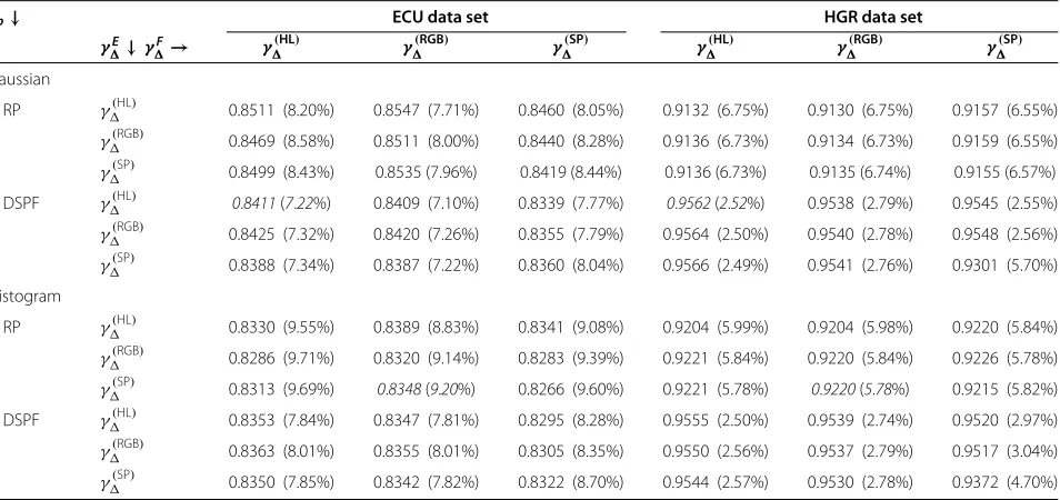
Table 3F-measure and minimal errorδmin(given in brackets) obtained using different local propagation costs
γp↓ ECU data set HGR data set
γE
↓γF→ γ(HL) γ(RGB) γ(SP) γ(HL) γ(RGB) γ(SP)
Gaussian
RP γ(HL) 0.8511 (8.20%) 0.8547 (7.71%) 0.8460 (8.05%) 0.9132 (6.75%) 0.9130 (6.75%) 0.9157 (6.55%) γ(RGB)
0.8469 (8.58%) 0.8511 (8.00%) 0.8440 (8.28%) 0.9136 (6.73%) 0.9134 (6.73%) 0.9159 (6.55%)
γ(SP)
0.8499 (8.43%) 0.8535 (7.96%) 0.8419 (8.44%) 0.9136 (6.73%) 0.9135 (6.74%) 0.9155 (6.57%)
DSPF γ(HL) 0.8411(7.22%) 0.8409 (7.10%) 0.8339 (7.77%) 0.9562(2.52%) 0.9538 (2.79%) 0.9545 (2.55%) γ(RGB)
0.8425 (7.32%) 0.8420 (7.26%) 0.8355 (7.79%) 0.9564 (2.50%) 0.9540 (2.78%) 0.9548 (2.56%)
γ(SP)
0.8388 (7.34%) 0.8387 (7.22%) 0.8360 (8.04%) 0.9566 (2.49%) 0.9541 (2.76%) 0.9301 (5.70%)
Histogram
RP γ(HL) 0.8330 (9.55%) 0.8389 (8.83%) 0.8341 (9.08%) 0.9204 (5.99%) 0.9204 (5.98%) 0.9220 (5.84%) γ(RGB)
0.8286 (9.71%) 0.8320 (9.14%) 0.8283 (9.39%) 0.9221 (5.84%) 0.9220 (5.84%) 0.9226 (5.78%)
γ(SP)
0.8313 (9.69%) 0.8348(9.20%) 0.8266 (9.60%) 0.9221 (5.78%) 0.9220(5.78%) 0.9215 (5.82%)
DSPF γ(HL) 0.8353 (7.84%) 0.8347 (7.81%) 0.8295 (8.28%) 0.9555 (2.50%) 0.9539 (2.74%) 0.9520 (2.97%) γ(RGB)
0.8363 (8.01%) 0.8355 (8.01%) 0.8305 (8.35%) 0.9550 (2.56%) 0.9537 (2.79%) 0.9517 (3.04%)
γ(SP)
0.8350 (7.85%) 0.8342 (7.82%) 0.8322 (8.70%) 0.9544 (2.57%) 0.9530 (2.78%) 0.9372 (4.70%) The arrows indicate the column or row. Italicized values indicate the configuration used in the remaining experiments.
that every image contains the skin (i.e., both thresholds are set to zero), thenδfpnsfor the HGR set is extremely high, while for ECU it is at a moderate level. This is because the images in the ECU set contain uncontrolled multi-colored background, while the background in many images from the HGR set is uniform. In such cases, after adaptation, the entire background is classified as skin, while for ECU only some objects in the background are misclassified. Overall, we useTseedP = 0.12 and TP
r = 0.24 (italicized in Table 2), which does not decrease the scores for skin images significantly, whileδfpnsis at an acceptable level.
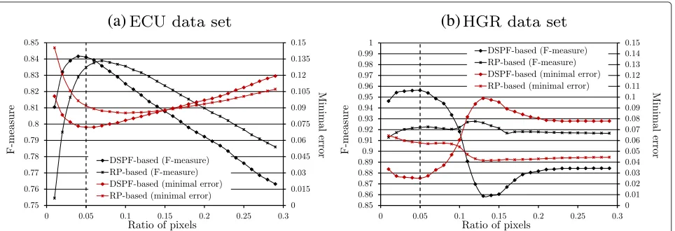
The scores obtained depending on theRseed ratio are presented in Figure 4. It can be seen from the plots that the algorithm is quite sensitive to this parameter; however,
in case of both data sets, the optimal value is around Rseed = 0.05 (marked with a vertical dashed line), and this value has been used in our experiments. In the case of the HGR set, the scores for the DSPF-based propaga-tion deteriorate whenRseed surpasses 0.05, but then (at about 0.15) they start improving again. In order to inves-tigate this, we measured the precision and potential recall in the seeds (the plots are presented in Additional file 2). We have found that for the HGR set, the potential recall in the initial and expanded seeds temporarily decreases (for Rseed ∈[0.1; 0.15]), because the true-positive blobs are eliminated due to the size-based filtering. However, for smaller values ofRseed, the size-based filtering helps achieve higher precision in the initial seeds.
(a)
(b)
Table 4F-measure and minimal errorδmin(given in brackets) obtained using different local skin color models
γp→ RP-based DSPF-based
↓Local skin color model ECU data set HGR data set ECU data set HGR data set Gaussian 0.8535 (7.96%) 0.9135 (6.74%) 0.8411(7.22%) 0.9562(2.52%)
Histogram, 256 bins 0.8308 (9.42%) 0.9215 (5.80%) 0.8347 (8.00%) 0.9556 (2.51%)
Histogram, 128 bins 0.8348(9.20%) 0.9220(5.78%) 0.8353 (7.84%) 0.9555 (2.50%)
Histogram, 64 bins 0.8400 (8.82%) 0.9217 (5.86%) 0.8348 (7.56%) 0.9563 (2.43%)
Histogram, 32 bins 0.8328 (9.01%) 0.9145 (6.59%) 0.8257 (7.90%) 0.9559 (2.49%)
Histogram, 16 bins 0.8107 (9.95%) 0.9134 (6.67%) 0.8125 (8.62%) 0.9533 (2.69%)
Histogram, 8 bins 0.7906 (10.96%) 0.9138 (6.67%) 0.7982 (9.62%) 0.9481 (3.06%)
The arrows indicate the column or row. Italicized values indicate the selected configuration.
In Table 3, we present the scores obtained using differ-ent local costs utilized to build the expanded seedsγE and to propagate the final ‘skinness’γF. The local skin color model was trained using either a single multivari-ate Gaussian, or using the color histogram with 128 bins per channel. It may be seen from the table that the RP-based propagation is more sensitive to the costs used, and different settings are optimal for the ECU and HGR sets. In some cases, theF-measure for the ECU set is higher using RP, but overall it is the DSPF-based propagation which delivers high scores for both the ECU and HGR
sets. The italicized values indicate the configuration used in the remaining experiments.
The seeds are expanded depending on the total path cost boundaryT, and the sensitiveness to this parame-ter is demonstrated in Figure 5. It may be observed that the scores are little dependent on this value, and we used T =3 in our experiments (marked with a vertical dashed line in the plots).
We have trained the local skin color model using a single multivariate Gaussian as well as using the color histogram with different numbers of bins per channel.
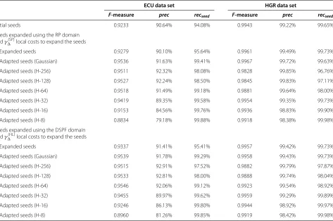
Table 5 Skin detection scores computed in the seeds at subsequent processing steps
ECU data set HGR data set
F-measure prec recseed F-measure prec recseed
Initial seeds 0.9233 90.64% 94.08% 0.9943 99.22% 99.65%
Seeds expanded using the RP domain andγ(SP)local costs to expand the seeds
Expanded seeds 0.9279 90.10% 95.64% 0.9961 99.49% 99.73%
Adapted seeds (Gaussian) 0.9536 91.63% 99.41% 0.9967 99.72% 99.63%
Adapted seeds (H-256) 0.9511 92.32% 98.08% 0.9828 99.85% 96.76%
Adapted seeds (H-128) 0.9527 92.24% 98.50% 0.9845 99.83% 97.11%
Adapted seeds (H-64) 0.9518 91.49% 99.18% 0.9881 99.64% 98.00%
Adapted seeds (H-32) 0.9419 89.35% 99.58% 0.9954 99.35% 99.73%
Adapted seeds (H-16) 0.9153 84.56% 99.76% 0.9936 98.83% 99.90%
Adapted seeds (H-8) 0.8834 79.18% 99.88% 0.9918 98.38% 99.98%
Seeds expanded using the DSPF domain andγ(HL)local costs to expand the seeds
Expanded seeds 0.9337 91.41% 95.41% 0.9957 99.42% 99.73%
Adapted seeds (Gaussian) 0.9539 91.78% 99.29% 0.9958 99.43% 99.73%
Adapted seeds (H-256) 0.9515 92.91% 97.52% 0.9882 99.79% 97.87%
Adapted seeds (H-128) 0.9533 92.81% 98.00% 0.9888 99.74% 98.04%
Adapted seeds (H-64) 0.9546 92.06% 99.12% 0.9923 99.54% 98.92%
Adapted seeds (H-32) 0.9455 89.97% 99.62% 0.9959 99.29% 99.89%
Adapted seeds (H-16) 0.9246 86.13% 99.80% 0.9944 98.92% 99.97%
Adapted seeds (H-8) 0.8960 81.26% 99.85% 0.9919 98.42% 99.98%
Table 6 Skin detection scores obtained using different methods for the ECU data set
Acceptance threshold Acceptance threshold
Method set to maximizeF-measure set to minimizeδmin
F-measure prec rec δnsfp δmin rec δfp δfpns
Global Bayesian classifier [16] 0.7772 73.15% 82.89% 9.13% 12.13% 89.27% 13.52% 13.52%
Global model in ESS [14] 0.7434 68.07% 81.88% 11.79% 14.13% 87.76% 16.03% 16.03%
Chen’s global model [15] 0.6896 55.30% 91.61% 23.11% 15.75% 91.61% 23.11% 23.11%
Wavelet-based hybrid detector [61] 0.7894 76.34% 81.73% 9.01% 12.28% 88.74% 13.31% 13.78%
Face-based adaptation in ESS [40] 0.7672 69.67% 85.35% - 13.95% 89.85% 17.74%
-Spatial analysis using RP [59] 0.8177 75.79% 88.78% 8.45% 9.87% 92.32% 12.06% 10.32%
Spatial analysis using DSPFs [9] 0.8303 78.09% 88.65% 9.06% 7.68% 93.28% 8.64% 12.08%
Face-based adaptive seeds [11] 0.8661 82.70% 90.92% - 7.17% 94.06% 8.39%
-Proposed method (RP-based) 0.8348 81.07% 86.04% 8.40% 9.20% 90.85% 9.25% 10.44%
Proposed method (DSPF-based) 0.8411 79.10% 89.79% 12.67% 7.22% 94.14% 8.57% 16.57%
Italicized values indicate the best score.
The obtained scores are presented in Table 4 (the itali-cized values indicate the selected configuration). For the ECU set, both RP-based and DSPF-based propagations deliver the best scores when the local model is learned with a Gaussian; however, in the case of RP, the scores for the HGR set are much worse than when using the histogram-based model. Also, analysis of the plots in Additional file 2 allows us to conclude that the Gaus-sian offers higher generalization than the histogram-based model.
Finally, in Table 5, we present the scores computed in the seeds at subsequent steps of their extraction. Here, we show the results for RP- and DSPF-based propagation, using different local costsγE. It may be seen that for the ECU set, the potential recall and theF-measure increase substantially between the initial and adapted seeds. In the case of the HGR set, the potential recall is high already in the initial seeds; as in many cases, there is a single skin blob in these images, and it is already covered by the initial seeds. Overall, it is clear that the scores improve during
the seed extraction process, which justifies its subsequent steps.
5.3 Quantitative comparison
The scores obtained using a number of alternative state-of-the-art methods are presented in Tables 6 and 7. ROC and precision-recall curves are rendered in Figures 6 and 7. In the case of the ECU set, we have included two face-based adaptation methods [11,40]. Naturally, they were omitted for the HGR images as they do not present human faces. In the tables, we demonstrate the scores for two values of the acceptance threshold, for which theF-measure is maximal and the errorδminis minimal, respectively.
The methods operating in the ESS [14,40] offer binary skin classification, but we extended them so that they pro-duce the continuous response. In the plots in Figures 6 and 7, each result for the original binary decision is indi-cated with a cross (obviously, it is positioned on the ROC or precision-recall curve).
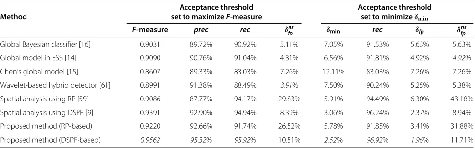
Table 7 Skin detection scores obtained using different methods for the HGR data set
Acceptance threshold Acceptance threshold
Method set to maximizeF-measure set to minimizeδmin
F-measure prec rec δfpns δmin rec δfp δfpns
Global Bayesian classifier [16] 0.9031 89.72% 90.92% 5.11% 7.05% 91.53% 5.63% 5.63%
Global model in ESS [14] 0.9090 90.76% 91.04% 4.31% 6.56% 91.81% 4.92% 4.92%
Chen’s global model [15] 0.8607 89.33% 83.03% 7.26% 12.11% 83.03% 7.26% 7.26%
Wavelet-based hybrid detector [61] 0.8991 91.38% 88.49% 3.91% 7.50% 90.24% 5.25% 5.38%
Spatial analysis using RP [59] 0.9086 87.77% 94.17% 29.83% 5.91% 94.49% 6.30% 43.18%
Spatial analysis using DSPF [9] 0.9391 92.90% 94.94% 8.39% 3.06% 96.24% 2.37% 8.94%
Proposed method (RP-based) 0.9220 92.66% 91.74% 26.52% 5.78% 91.85% 3.41% 31.88%
Proposed method (DSPF-based) 0.9562 95.32% 95.92% 10.51% 2.52% 96.92% 1.96% 11.71%
(a)
(b)
(a)
(b)
The method utilizing the face-based adaptive seeds [11] delivers the best scores for the ECU set, especially in terms of the precision-recall and the F-measure. The ROC curve and minimal error δmin are virtually identi-cal with those obtained with our DSPF-based approach. However, it must be noted that this method requires addi-tional information delivered by a face detector. Here, we carefully selected those images, in which the faces are correctly detected, in order to demonstrate the maxi-mal advantage that can be achieved using the face-based adaptation over the proposed self-adaptive method. The second face-based adaptation technique, which operates in ESS, improves the global skin color model in ESS, but it is not competitive compared with other techniques. For the HGR set, our adaptation scheme with DSPF-based propagation outperforms other methods, offering very high skin segmentation accuracy (F-measure is 0.9562 and
δmin=2.52%).
We have also measured the false-positive rate(δnsfp)for images that do not present human skin. As it was already mentioned, we used the same ECU and HGR images, in which the skin regions were excluded from process-ing, and we applied the same values of the acceptance threshold as in the case of the original images. In this way, we investigated whether and how the absence of skin regions influences the false-positive rate. This experiment was not executed for the face-based adaptation schemes, because after excluding the skin regions, the faces should not be detected at all. Obviously, for pixel-wise classifica-tion schemes, the false-positive rate is identical regardless of whether the skin is present in the image. For other methods, the false-positive rate is generally higher, as each of them adapts to some extent to the image. Overall, using the self-adaptive seeds with the DSPF-based propagation domain (the RP-based domain is more sensitive here),δnsfp is from 3.05% (ECU, δmin) to 6.08% (HGR,δmin) higher than obtained with the Bayesian classifier. This shows that the incorrect adaptation is a potential problem; however, we managed to limit its impact using a simple image-level skin detector. Also, this problem is common to all the adaptive methods, including the face-based schemes in case of false-positive face detection. Last, but not least, there are many applications, including hand pose estima-tion, where efficient skin segmentation is critical, and such errors can be mitigated at further processing stages (e.g., a hand shape would be unlikely to be matched, if the entire detected skin region is falsely-positive).
The average processing times required to process a 512×512 image are quoted in Table 8. It may be observed that almost half of the computation time (i.e., 216.6 ms) is consumed to create the adaptive seeds. When a video stream is processed, the adaptation does not have to be performed for every frame as the scene usually does not change with a high frequency rate. This means that the
Table 8 Average processing times for a 512×512 image
Method Time (ms)
Global Bayesian classifier [16] 5.2
Global model in ESS [14] 4.8
Chen’s global model [15] 0.8
Wavelet-based hybrid detector [61] 4,952.5
Face-based adaptation in ESS [40] 24.1
Spatial analysis using RP [59] 92.9
Spatial analysis using DSPF [9] 361.1
Face-based adaptive seeds [11] 130.5
Proposed method (RP-based) 232.9
Skin detection using global model 5.29
Skin seeds initialization 56.34
Expansion of the seeds 77.97
Adaptation of the seeds 19.49
Final spatial analysis 73.81
Proposed method (DSPF-based) 548.2
Skin detection using global model 5.34
Generation of the DSPF skin map 192.43
Skin seeds initialization 46.18
Expansion of the seeds 79.30
Adaptation of the seeds 91.17
Final spatial analysis 133.78
skin model can be adapted once for a given scene and then the stream can be processed at ca. three frames per second. Also, it may be seen that the RP-based propaga-tion is much faster, because (i) the DSPF skin map does not have to be computed and (ii) the histogram-based adaptation is much faster than using a Gaussian model. Excluding the adaptation phase, the RP-based approach requires 79.1 ms, which allows processing over 12 frames per second. Overall, there are two time-consuming oper-ations which could potentially be optimized, namely (i) generation of the DSPF skin map and (ii) the distance transform. The former includes a number of independent operations (the basic features are computed in several ker-nels), which may be executed in parallel to reduce the processing time. The main problem with the distance transform lies in non-linear access to the memory while processing the pixels popped from the priority queue used in the Dijkstra algorithm. Possibly, this may be improved by including the neighborhood criteria into the priority measure to avoid referring to the pixels far from each other in the memory, but this needs to be investigated.
5.4 Qualitative comparison
(a)
(b)
(c)
(d)
(e)
(f)
(g)
(h)
Figure 8Examples of skin segmentation for the ECU data set obtained using different methods.The presented images come from the publicly available ECU benchmark data set [65].
skin regions with high precision. Images IX and X are the examples of incorrect adaptation. Here, the background has a skin-like color, and the seeds are detected both in the skin, and in the background, resulting in very high false-positive errors. However, it is worth mentioning that the alternative detectors fail in these cases as well, except
(a)
(b)
(c)
(d)
(e)
(f)
Figure 9Examples of skin segmentation for the HGR data set obtained using different methods.The presented images come from the HGR data set [9].
appear inside the facial region, leading to incorrect adap-tation. Naturally, this problem does not appear in our self-adaptive approach.
For the HGR images presented in Figure 9, our DSPF-based method offers almost perfect skin segmentation, and it clearly outperforms all the alternative algorithms. Also, comparing the results with [9], it is evident that using the adaptive seeds is more effective than the threshold-based seeds extraction.
6 Conclusions
In this paper, we proposed a new method for creating self-adaptive seeds for spatial-based skin segmentation. From the seeds, the ‘skinness’ is propagated either using the raw
skin probability obtained from a global skin color model or using the probability computed in the DSPF space. Our extensive experimental study demonstrated that the DSPF domain is less sensitive to the method’s parameters and outperforms all of the investigated methods both for the ECU and HGR data sets, except for our earlier face-based adaptation [11]. The raw probability domain is much more sensitive, which makes it difficult to tune; however, in some cases (for the ECU set), it delivered better results than the DSPF and also it is much less time consuming. Overall, we found it worth being reported as well.
over the face-based adaptation schemes, and we demon-strated that using the self-adaptive seeds, it is possible to obtain results comparable with the face-based adaptation. The benefits in case of images that do not present human faces are obvious, while there are also many examples presented in the paper, when the proposed adaptation method outperforms the face-based ones.
Our current research plans include combining the intro-duced adaptation technique with the face-based schemes, which may help in cases when the background pixels appear in the detected facial regions. Furthermore, we intend to improve the image-level skin detection; we have demonstrated in our experimental study that this is an important, while often disregarded, problem in adaptive skin color modeling. Last, but not least, the algorithm should be parallelized and optimized in order to make it suitable for processing video sequences.
Additional files
Additional file 1: Packed text files.The files contain the names of the files used in the training and test set.
Additional file 2: Supplementary figures.The figures illustrate the detection accuracy in the skin seeds obtained with different ratios of the pixelsRseedused to build the initial seeds.
Competing interests
The authors declare that they have no competing interests.
Acknowledgements
This work was supported by the Polish National Science Center (NCN) under the Grant: DEC-2012/07/B/ST6/01227. This work was performed using the infrastructure supported by POIG.02.03.01-24-099/13 grant: ‘GeCONiI’ Upper Silesian Center for Computational Science and Engineering. JK was supported by the European Union from the European Social Fund (grant agreement number: UDA-POKL.04.01.01-00-106/09).
Received: 16 July 2014 Accepted: 27 October 2014 Published: 29 November 2014
References
1. P Kakumanu, S Makrogiannis, NG Bourbakis, A survey of skin-color modeling and detection methods. Pattern Recogn.40(3), 1106–1122 (2007)
2. M Kawulok, J Nalepa, J Kawulok, inLecture Notes in Computational Vision and Biomechanics: Advances in Low-Level Color Image Processing,vol. 11, ed. by ME Celebi, B Smolka. Skin detection and segmentation in color images (Springer, Netherlands, 2014), pp. 329–366
3. S Bilal, R Akmeliawati, MJE Salami, AA Shafie, Dynamic approach for real-time skin detection. J. Real-Time Image Process (2012). doi:10.1007/s11554-012-0305-2
4. J-S Lee, Y-M Kuo, P-C Chung, E-L Chen, Naked image detection based on adaptive and extensible skin color model. Pattern Recognit.
40, 2261–2270 (2007)
5. H Kruppa, MA Bauer, B Schiele, inLecture Notes in Computer Science: Pattern Recognition,vol. 2449, ed. by L Van Gool. Skin patch detection in real-world images (Springer, Berlin, 2002), pp. 109–116
6. M Silveira, JC Nascimento, JS Marques, ARS Marcal, T Mendonca, S Yamauchi, J Maeda, J Rozeira, Comparison of segmentation methods for melanoma diagnosis in dermoscopy images. IEEE J. Selected Topics Signal Process.3(1), 35–45 (2009)
7. H Castillejos, V Ponomaryov, L Nino-de-Rivera, V Golikov, Wavelet transform fuzzy algorithms for dermoscopic image segmentation. Comput. Math. Methods Med.2012, 578721 (2012)
8. B Choi, B Chung, J Ryou, inProceedings of the International Conference on Computer Sciences and Convergence Information Technology (ICCIT). Adult image detection using Bayesian decision rule weighted by SVM probability (Seoul, Korea, 2009), pp. 659–662
9. M Kawulok, J Kawulok, J Nalepa, Spatial-based skin detection using discriminative skin-presence features. Pattern Recogn. Lett.41, 3–13 (2014)
10. R Khan, A Hanbury, J Stöttinger, A Bais, Color based skin classification. Pattern Recogn. Lett.33(2), 157–163 (2012)
11. M Kawulok, J Kawulok, J Nalepa, M Papiez, inProceedings of the IEEE International Conference on Image Processing (ICIP). Skin detection using spatial analysis with adaptive seed (Melbourne, Australia, 2013), pp. 3720–3724
12. J Kovac, P Peer, F Solina, Human skin color clustering for face detection. EUROCON2, 144–148 (2003)
13. J-C Terrillon, M David, S Akamatsu, inProceedings of the International Conference on Automatic Face and Gesture Recognition. Automatic detection of human faces in natural scene images by use of a skin color model and of invariant moments (Nara, Japan, 1998), pp. 112–117 14. A Cheddad, J Condell, K Curran, P Mc Kevitt, A skin tone detection
algorithm for an adaptive approach to steganography. Signal Process.
89(12), 2465–2478 (2009)
15. Y-H Chen, K-T Hu, S-J Ruan, Statistical skin color detection method without color transformation for real-time surveillance systems. Eng. Appl. Artif. Intell.25(7), 1331–1337 (2012)
16. MJ Jones, JM Rehg, Statistical color models with application to skin detection. Int. J. Comput. Vis.46, 81–96 (2002)
17. SL Phung, A Bouzerdoum, D Chai, Skin segmentation using color pixel classification: analysis and comparison. IEEE Trans. Pattern Anal. Mach. Intell.27(1), 148–154 (2005)
18. T Chaira, AK Ray, Fuzzy approach for color region extraction. Pattern Recognit. Lett.24(12), 1943–1950 (2003)
19. H Greenspan, J Goldberger, I Eshet, Mixture model for face-color modeling and segmentation. Pattern Recognit. Lett.22, 1525–1536 (2001) 20. TS Caetano, SD Olabarriaga, DAC Barone, Do mixture models in
chromaticity space improve skin detection? Pattern Recognit.
36, 3019–3021 (2003)
21. SL Phung, A Bouzerdoum, D Chai, inProceedings of the International Conference on Image Processing (ICIP),vol. 1. A novel skin color model in YCbCr color space and its application to human face detection, (2002), pp. 289–292
22. M-J Seow, D Valaparla, VK Asari, inProceedings of the Applied Imagery Pattern Recognition Workshop. Neural network based skin color model for face detection, (2003), pp. 141–145
23. KK Bhoyar, OG Kakde, Skin color detection model using neural networks and its performance evaluation. J. Comput. Sci.6(9), 963–968 (2010) 24. M Kawulok, J Nalepa, inLecture Notes in Computer Science: Structural,
Syntactic, and Statistical Pattern Recognition,vol. 7626, ed. by G Gimel’farb, E Hancock, A Imiya, A Kuijper, M Kudo, S Omachi, T Windeatt, and K Yamada. Support vector machines training data selection using a genetic algorithm (Springer, New York, 2012), pp. 557–565
25. J Han, G Awad, A Sutherland, H Wu, inProceedings of the IEEE International Conference on Automatic Face and Gesture Recognition. Automatic skin segmentation for gesture recognition combining region and support vector machine active learning (IEEE Computer Society, Washington D.C., 2006), pp. 237–242
26. ME Celebi, HA Kingravi, H Iyatomi, Y Alp Aslandogan, WV Stoecker, RH Moss, JM Malters, JM Grichnik, AA Marghoob, HS Rabinovitz, SW Menzies, Border detection in dermoscopy images using statistical region merging. Skin Res. Tech.14(3), 347–353 (2008)
27. ME Celebi, H Iyatomi, G Schaefer, WV Stoecker, Lesion border detection in dermoscopy images. Comput. Med. Imag. Graph.33(2), 148–153 (2009) 28. Q Abbas, ME Celebi, I Fondón García, M Rashid, Lesion border detection
in dermoscopy images using dynamic programming. Skin Res. Tech.
17(1), 91–100 (2011)