A Comparison and Improvement of Online Learning Algorithms for Sequence Labeling

A Comparison and Improvement of Online Learning

Algorithms for Sequence Labeling

Zheng yan He Hou f eng Wang

Key Laboratory of Computational Linguistics (Peking University) Ministry of Education,China [email protected], [email protected]

A

Sequence labeling models like conditional random fields have been successfully applied in a variety of NLP tasks. However, as the size of label set and dataset grows, the learning speed of batch algorithms like L-BFGS quickly becomes computationally unacceptable. Several online learning methods have been proposed in large scale setting, yet little effort has been made to compare the performance of these algorithms. Comparison is often carried out on a few datasets with fine tuned parameters for specific algorithm. In this paper, we investigate and compare several online learning algorithms for sequence labeling with datasets varying in scale, feature design and label set. We find that Dual Coordinate Ascent (DCA) is robust across datasets even without careful tuning of parameter. Furthermore, a recently proposed variant of Stochastic Gradient Descent (SGD), Adaptive online gradient Descent based on feature Frequency information (ADF), has very fast training speed compared with plain SGD, but fails to converge under certain conditions. Finally, We propose a simple modification of ADF, which bears comparable convergence speed with ADF, and is consistently better than plain SGD.

T

A

C

　序

序

序

列

列

列

标

标

标

注

注

注

在

在

在

线

线

线

学习

学

学

习

习

算

算

算

法

法

法

的

的

的

比

比

比

较

较

较

和

和

和改

改

改

进

进

进

序列标注模型，如条件随机场，已广泛用于自然语言处理的很多任务中。但随着数 据规模和标记集的增大，批量学习算法（如L-BFGS）的训练时间复杂性变得越来越不可接

受；于是，出_现了多_个大_规模_{环境下的在线学习}算法_。这_些算法_有各自_的特_点，但对这_些 算法_的比较_研究很少_有报_道。通常情况_{下都是针对}几_{个数据集，通}过_对特_定算法_细致调 整参数来比较_{最后的测试结果。本文针对}几_个典_{型的序列标}注_在线学习算法_{，在不同规} 模_、特征_{设计和标记集合的数据集上}进_行了比较_研究_{。结果发现，即使}没_有特_别对参数

调_{优，对偶坐标上升}算法_{（DCA）在不同数据集上也能有}很好_{的表现；而随机梯度下降}

算法_（SGD）的一个变种算法_——基于特征频_度的适应性_{在线梯度下降}法_（ADF）与普通

的SGD相比_{，训练速度更}快_{，但不能保证}总_{收敛。最后，本文}还_对ADF提出_了一种简_单的 改进_，改进_后的算法好_{于普通的SGD，与ADF收敛速度接}近_。

K

:

K

C

:

1 Introduction

Sequence labeling models have been widely used in a variety of NLP tasks, such as word segmentation, part-of-speech tagging, chunking, and named entity recognition. Various se-quence labeling models have been proposed, like hidden Markov models (HMM) (Rabiner, 1989), structured perceptron (Collins, 2002), conditional random fields (CRFs) (Lafferty et al., 2001) and SVM-HMM (Tsochantaridis et al., 2006). In recent years, discriminative models gain significant popularity over generative models on these tasks, and achieve state-of-the-art performance on most above tasks. Their strength and flexibility come from their ability to incorporate arbitrary declarative features.

CRFs is one of such discriminative models for sequence labeling built upon maximum entropy principle. The learning algorithms of CRFs can be divided into batch methods and online methods. Batch methods update parameters by estimating gradient over the entire training data, while online methods estimate noisy gradient with a small portion of the training data, and update parameters frequently. Among all the batch methods, L-BFGS is the most widely used and outperforms others by a substantial margin (Malouf et al., 2002); Conjugate-gradient (CG) method with proper preconditioner can converge as fast as L-BFGS (Sha and Pereira, 2003). However, discriminative models for typical sequence labeling tasks are very large and may involve hundreds of thousands of features, rendering even fastest batch learning methods very slow and impractical for large scale datasets.

Several online learning algorithms have been proposed to speed the training process of struc-tured prediction problems, such as Passive-Aggressive (PA) algorithm (Crammer et al., 2006), Dual Coordinate Ascent (DCA) (Martins et al., 2010) and Stochastic Gradient Descent (SGD). SGD is known for its performance in the back propagation training of neural network. It also shows extremely good performance on machine learning tasks such as SVM (Bordes et al., 2009), CRFs (Vishwanathan et al., 2006), and Markov Logic Networks (Poon and Vanderwende, 2010). It may reach optimal performance even before it sees the whole training data on large datasets (Bottou and Bousquet, 2008). SGD takes typically 5-10 iterations to converge when training a multiclass Maximum Entropy (ME) model, while it takes over 50 iterations when training CRFs, much slower than training its unstructured counterpart, multiclass ME. We show how simple feature frequency adaptive strategy may help accelerate training of CRFs within 10 iterations.

Despite recent progresses in online learning algorithms, little effort has been made to compare these algorithms thoroughly. In this paper, we focus on several online learning algorithms for sequence labeling. More specifically, we investigate PA, DCA, SGD and SGD’s variant ADF (Sun et al., 2012). We perform comparison on several standard datasets with diverse settings of feature design and label set. We make it as close as possible to real application scenarios whenever resources are available. Experiment reveals distinct behavior of these algorithms under different settings.

The remaining of this paper is organized as follows: in Section 2, we describe in detail the online learning algorithms, and propose MADF; in Section 3 we evaluate performance of these algorithms, and present novel usage of Tongyici Cilin (Extended) in Experiment 2; we review related work in Section 4; finally we conclude.

2 Online Learning Algorithms for Sequence Labeling

A sequence labeling task is defined as follows: given an observation sequence x = {x1,x2, . . . ,xn}, output its corresponding label sequencey={y1,y2, . . . ,yn}, one label for eachxi. The output space is|Y|nwhereY is the label set that each individualyitakes values from, andnis the length ofy.

In discriminative sequence labeling models, feature functions are used to describe interde-pendency between observed and hidden variables. Under first order Markov assumption, the feature function can be divided into transition featuresφ(x,yi,yi+1)and emission features

φ(x,yi). These can be combined toφ(x,y).

Dynamic programming technique like viterbi decoding is often employed during inference:

ˆ

y=arg max

y θ

T_{φ(x,y) (1)}

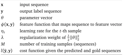
whereθ are model parameters. Next we will describe how to estimate parametersθ with different online algorithms. Table 1 shows a list of denotations for convenience.

x input sequence

y output label sequence

θ parameter vector

φ(x,y) feature function that maps sequence to feature vector

ηt learning rate for thet-th sample

λ regularization weight ofλ₂kθk2 2

M number of training samples (sequences)

l(ˆy,y) cost function given the predicted and gold sequences

Table 1: Denotations

2.1 Passive-aggressive algorithm (PA)

Passive-Aggressive (PA) algorithm (Crammer et al., 2006) is a family of margin based online learning algorithms. This algorithm updates the parameter to satisfy the constraint imposed by the current example (aggressively), and does nothing if the current example is correctly classified (passively). Equation 2 defines the objective function for PA algorithm (referred by the author as PA-I):

θ(t+1)_{=arg min}

θ 1

quality. The update rule of parameter is as follows:

θ(t+1)_=θ(t)_−η(φ(x(t)_,ˆy(t)_)−φ(x(t)_,y(t)_{)) (3)}

where η=minC,θ

T_(φ(x(t)_,ˆy(t)_)−φ(x(t)_,y(t)_{)) +l(y}(t)_,ˆy(t)₎

kφ(x(t)_,ˆy(t)_)−φ(x(t)_,y(t)_)k2 (4) and ˆy(t)_{=arg max}

y θ

T_(φ(x(t)_,y)−φ(x(t)_,y(t)_{)) +l(y}(t)_{,y) (5)}

wherel(y(t)_,ˆy(t)_{)is the penalty we incur if our prediction isyˆ}(t)_{and the true label isy}(t)_.ˆy(t)

can be solved with cost augmented decoding, which can be efficiently accomplished ifl(y(t)_,yˆ(t)₎

decomposes the same way as the feature vector function (Smith, 2011). This is referred to as a max-loss update in (Crammer et al., 2006).

When applied to sequence labeling PA is a special case of the general algorithm where outputy

is a label sequence. Hamming loss (Eq. 6) is often used. However, other loss can also fit when one faces with task specific needs (Song et al., 2012) (Mohit et al., 2012).

l(ˆy,y) =Hamming(ˆy,y) =

n X

i=1

δyi6=ˆyi(ˆyi,yi) (6)

2.2 Dual coordinate ascent (DCA)

(Martins et al., 2010) present a general framework for online learning of structured classifiers. It bears some resemblance to the PA algorithm in that it shares the passive-aggressive property of PA. This algorithm applies to a wide class of loss functions; CRFs, SVM, structured perceptron can all be deemed as its special cases. Furthermore, learning rate is automatically determined for each instance, hence pesky learning rate tuning is no longer needed. The learning objective is the sum of loss on datasets plus a regularization term:

min θ∈RdλR(θ) +

1

m

m X

t=1

L(θ;x(t)_,y(t)_{) (7)}

The update rule 8 is very similar to the PA algorithm in large margin setting (Eq. 3), if we divide Equation 7 byλ, replace 1

λmwithC, and set∇L=φ(x(t),ˆy(t))−φ(x(t),y(t)). The update rule for DCA is:

θ(t+1)_=θ(t)_−η

t∇L(θ;x(t),y(t)) (8)

where η(t)_=min 1 λm,

L(θ(t)_;x(t)_,y(t)₎

k∇L(θ(t)_;x(t)_,y(t)_)k2 (9) As for sequence labeling problem, CRFs is derived by setting the loss function to the negative log-loss with no cost function, i.e. LCRF=−logP(yt|xt). The loss function of CRFs is just a special case of the general loss functionL.

2.3 CRFs with SGD learning and its variants

Linear chain conditional random fields (CRFs) (Lafferty et al., 2001) is widely used model for sequence labeling. It predicts the output sequenceyby its conditional probabilityP(y|x):

P(y|x) =_Z1 (x)expθ

whereZ(x) =P_yexpθTφ(x,y)is normalization term which ensures that the probability sums to 1. The training objective is to maximize the likelihood on the training data (often accompanies a prior over parameters to get max-a-posterior estimation), which is equivalent to minimizing a negative log loss over all data points plus a regularizer:

L=

m X

i=1

−logP(y|x) +λmkθk2 ₍₁₁₎

Here we multiply the regularizer bymto keep it consistent with Equation 7. This wayλhas the same meaning as in Equation 7. Minimizing this objective gives the gradient for one instance in online setting:

∂ ∂ θL(θ;x

(t)_,y(t)_{) =E}

P(y|x;θ(t)₎φ(x(t),y(t))−φ(x(t),y(t)) +λθ (12) where the expectation of feature vector given current examplex(t)_{is taken over all possible}

sequences ofy, and can be efficiently computed using forward-backward algorithm. Generally regularizer is added to avoid overfitting. Various regularizers have been proposed.L₂

regularizer,R(θ) =λ

2kθk22, which is used by various CRF based tools, often leads to superior performance and can be numerically optimized.L1regularizer,R(θ) =σkθk1, known as Lasso, encourages sparse parameter. Elastic net, a linear interpolation ofL₁andL₂regularizer, is used by (Lavergne et al., 2010) to regularize CRFs, and performs as good asL2regularizer, while still retaining compact model.

2.3.1 SGD and its variants

Stochastic gradient descent (SGD) is known for its fast convergence on machine learning tasks (Bottou and Bousquet, 2008) (Vishwanathan et al., 2006) (Shalev-Shwartz et al., 2007). Every time the algorithm randomly draws one sample (or small batch of samples in mini-batch setting), and performs update according to the gradient of this sample. In general, SGD has the following simple update rule:

θ(t+1)_=θ(t)_−η(t)_{B∇L (13)}

whereη(t)_{is a scalar learning rate,Bis a matrix;B=Ifor a plain SGD andB≈H}−1_{for second} order SGD. Despite its ease of implementation, it’s generally hard to tune and schedule the learning rate properly.

(Murata, 1998) shows that with a 1/t-annealing learning rate it can be asymptotically as effective as batch learning in terms of generalization error. (Bottou and Bousquet, 2008) further shows that utilizing second order information by settingηB=1_tH−1, optimal asymptotic

convergence rate is achieved. Withη=1/tand fixedB, convergence is guaranteed based on the theory of stochastic approximation (Murata, 1998).

2.3.2 ADF

In ADF, instead of a single global learning rate in plain SGD, each dimension of parameters has its own learning rate. The learning rate decays periodically according to its associated feature frequency, with high frequency decaying faster. This adaptive strategy is based on the intuition that frequent observed features are more adequately trained so smaller learning rates are needed. The author shows its high convergence speed compared with plain SGD in Chinese word segmentation task.

The method works well in most of our experiments, except for a few datasets. As we observed in our experiments in several other sequence labeling tasks, despite its speed of convergence and of reduction in training set error rate, it might fail to generalize well to testset and its parameters fluctuate a lot with different random shuffling of data. Moreover, it is not clear how to tune the upper bound and lower bound of the decay factor. In fact, ADF can be seen as diagonal approximation of the inverse of Hessian with exponential decrease learning rate based on frequency adaptive information. Unfortunately, this decrease in learning rate does not have theoretically convergence guarantee for now, although it works well in practice. (Murata, 1998) shows that SGD with 1/t-annealing learning rate guarantees convergence.

2.4 Modified ADF (MADF)

Second order SGD (2SGD) uses an approximation of inverse of Hessian by settingηB=1_tH−1

in order to achieve the optimal learning rate. Inspired by ADF and current theory foundation of 2SGD, we propose to use feature frequency information to approximateH−1_{, while still keeping} aη=1/tannealing factor, so convergence is guaranteed (Eq. 14).

Our method works as follows: at the beginning of the algorithm, we compute the diagonal scaling matricesBusing Equation 15, which is of the same size as the parameter vector. For each dimension ofθ, we use a separate learning rate1_tBii.

θ(t+1)_=θ(t)₋1

tB∇L(θ) (14)

Bii=

1

β+ (α−β)×#φ(x,y)

#tokens

where a=1 αb=

1

β (15)

whereaandbserve as lower and upper bounds of diagonal scaling elementBii. We keep

Bconstant during the training process. #φ(x,y)/#tokensis the relative feature frequency associated withi-th dimension.

There are two main differences of our method compared with ADF. The first is how the frequency is counted. In ADF, frequency is counted asP_yφ(x,y)per sentence and is the same for each

predicatexwith different y. Our method countsφ(x,y)per token in the training set and use separate learning rate for predicatexwith differenty. Another difference is that we keep an annealing learning rateη(t)_{=1/twith fixed diagonal scaling matrixB, while ADF can be seen}

as exponential decayingBwith constantη.

It is difficult to set the upper and lower bounds of scaling factorBii. One solution is to grid searchaandbwith held-out dataset. In this paper, we find it works surprisingly well by setting

It is easy to interpret our method in the view of input rescaling. In the back propagation learning of neutral network, mapping a too large input to a relatively small output would result in a small learning rate in order to ensure stable convergence, leading to slow convergence speed1_{. (LeCun et al., 1998) suggest simply to normalize the input to combat this problem.} Furthermore, input scaling is closely related to diagonal approximation of the inverse of Hessian (Bordes et al., 2009). However, scaling input feature value in sparse dataset is not realistic. Our idea is that in batch setting, the update of parameters associated with frequent features tend to be larger than those associated with rare features, so we scale the learning rate by the inverse of its associated relative feature frequency.

We show in Section 3 how this simple adaptive learning rate can significantly speedup the learning process while still is equipped with convergence guarantee. It runs as fast as plain SGD in terms of per iteration execution time, without the penalty of approximating the inverse of Hessian. The speedup is attributed to a proper estimation of initial learning rate, especially on datasets with more skewed feature frequency distribution.

3 Evaluation and Analysis

3.1 Implementation

There are several implementation issues on how to obtain good performance with different algorithms.

Weight averaging: averaged perceptron, PA and DCA can get much better performance by weight averaging. We only have to maintain two weight vectorsθ(t)_andθˆ(t)_{; each time we}

perform updateθ(t+1)_=θ(t)_{− ∇Landθˆ}(t+1)_{= ˆθ}(t)_{−t∇L. Finally the average weight is}

obtained by ¯θ=PTt=0θ(t)=θ(T)−θˆ(T)/T.

Randomize data: if we have to pass the dataset multiple times, it’s better to randomize the dataset. This can get better performance on all online algorithms in our experiments, not only SGD variants.

Regularization withL2: In NLP tasks, the feature vector is typically sparse. The gradient

∇L(see Eq. 12) consists of two parts, one corresponds with the loss and the other with the regularizer. The first part is often sparse and can be efficiently carried out. The update of the regularizer part is dense and quite expensive if done for every sample.

There are two methods that can combat this problem. (Shalev-Shwartz et al., 2007) propose to represent the weight vectorθ by the product of one scaling factor and one vector. We

can see the reason by a simple rearrangement of the formulaθ(t+1)_=θ(t)_{−η(∇l+λθ}(t)_{) =} (1−ηλ)θ(t)_{−η∇l. The first term can be done efficiently with a scalar product. (Bordes et al.,}

2009) propose in SVMSGD2 another method in which the regularizer term is treated as a special example and updated periodically. The method works on both first order and second order SGD. We will use this method in our experiment if not particularly mentioned.

Initial learning rate for SGD: The initial learning rate of SGD plays a critical role in the whole process of learning. It is chosen by heuristic method. We can sample a subset of the training data, run SGD algorithm for one pass over the subset and pick the learning rate with smallest training objective value as the initial guess of learning rate. This method is generally helpful for all SGD variants. We use this setting for all variants of SGD.

1_http:

3.2 Datasets settings

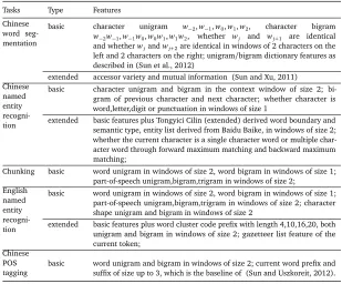
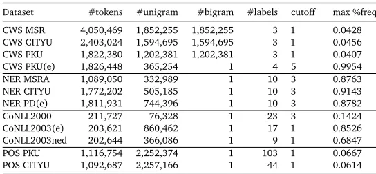
We compare the performance on several sequence labeling tasks, namely Chinese word seg-mentation, Chinese named entity recognition, CoNLL 2000 chunking, CoNLL 2003 NER, and Chinese part-of-speech tagging. The datasets vary across tasks in label set size and feature design. We inject as much knowledge as possible to mimic real application scenarios. For under-resourced tasks, we simply use token based n-gram features. Table 2 gives a brief view of features used. Table 4 shows the statistics after feature generation.

Tasks Type Features Chinese

word seg-mentation

basic character unigram w−2,w−1,w0,w1,w2, character bigram w−2w−1,w−1w0,w0w1,w1w2, whether wj and wj+1 are identical and whetherwjandwj+2are identical in windows of 2 characters on the left and 2 characters on the right; unigram/bigram dictionary features as described in (Sun et al., 2012)

extended accessor variety and mutual information (Sun and Xu, 2011) Chinese

named entity recogni-tion

basic character unigram and bigram in the context window of size 2; bi-gram of previous character and next character; whether character is word,letter,digit or punctuation in windows of size 1

extended basic features plus Tongyici Cilin (extended) derived word boundary and semantic type, entity list derived from Baidu Baike, in windows of size 2; whether the current character is a single character word or multiple char-acter word through forward maximum matching and backward maximum matching;

Chunking basic word unigram in windows of size 2, word bigram in windows of size 1; part-of-speech unigram,bigram,trigram in windows of size 2;

English named entity recogni-tion

basic word unigram in windows of size 2, word bigram in windows of size 1; part-of-speech unigram,bigram,trigram in windows of size 2; character shape unigram and bigram in windows of size 2

extended basic features plus word cluster code prefix with length 4,10,16,20, both unigram and bigram in windows of size 2; gazetteer list feature of the current token;

Chinese POS tagging

basic word unigram and bigram in windows of size 2; current word prefix and suffix of size up to 3, which is the baseline of (Sun and Uszkoreit, 2012).

Table 2: Features used for different tasks. For basic features, I refer to most simple token based feature and word type (letter,digit,punctuation) within a window of certain size. Extended features vary with available resources.

1.Chinese Word Segmentation (CWS)SigHan 2005 dataset is used for CWS2_.

2.Chinese Named Entity Recognition (NER)Named entity recognition requires large amount of world knowledge. List lookup features from gazetteer, lexicon and dictionaries can greatly enhance an NER system (Nadeau and Sekine, 2007). So for extended features, we explore the use of Baidu Baike and Tongyici Cilin (Extended)3_{as two knowledge} 2_{http://www.sighan.org/bakeoff2005/}

3_http:

sources. Table 3 gives a brief view of Tongyici Cilin. The first column gives the category

Category Word Cluster

Af10B05# 省长(governor of province)市长(mayor)县长(county head)区长乡长村长. . .

Ae13A10# 教教教授授授(professor) 副教授(associate professor)讲师(instructor)助教(teaching assistant) . . .

Hg05A01= 讲课 授课 讲授讲解教教教授授授(teach)教书. . .

Dm01A46# 安全_部(ministry of security)财政部(ministry of finance)参谋_部电力部. . .

Table 3: A Snippet from Tongyici Cinlin (Extended)

one word belongs to. The category codes with prefix of different lengths give different levels of abstraction of its semantic meaning. Some of the clusters are good indicators of named entities. For instance, the first row is a good indicator of previous word being a location, and the first and second row is a good indicator of next word being a person. This categorized lexicon is quite similar to word cluster features in (Ratinov and Roth, 2009), but is more precise. However, to our certain knowledge, this resource remains unexplored in previous Chinese NER tasks.

Words in Chinese do not have space like in English. In Chinese NER task, texts are given without word boundaries, so segmentation is an essential preprocessing step. But this will bring segmentation error to the system, especially most named entities are out-of-vocabulary words. On the other hand, if we perform inference at character level directly, we quickly loss the meaning of words . We propose two simple strategies to alleviate these problems: first, while still performing inference at character level, we do forward maximum matching and backward maximum matching to provide basic word boundary features; second, word meaning is injected with the category of the matching word in Tongyici Cilin. The class of a word also serves as a mechanism of word cluster, which holds similar words together. Hence Tongyici Cilin serves as both word clusters and a lexicon when performing maximum matching.

Finally, we use entity list extracted from Baidu Baike as additional entity list features. The datasets we use are SigHan 08 Chinese NER dataset and one month of People Daily. As our main concern is to build a resource rich feature design for Chinese named entity recognition, we do not make further comparison with other algorithms. Other approaches typically use complex model combinations, which are not directly comparable to our single model based method.

3.CoNLL English NER and Chunking (Ratinov and Roth, 2009) perform an extensive study on NER and extract valuable resources, which can be readily incorporated into any existing NER system. We use the word class hierarchy and gazetteer lists from their package4_{. We do not use other features for simplicity. Word class features are derived} from brown clustering algorithm and intended for bridging the gap of unseen text . The brown algorithm hierarchically clusters the words, and paths with different lengths to the root represent different levels of abstraction. Gazetteers are dictionaries of named entities and injected to the system to provide world knowledge. We use these two features as described in (Ratinov and Roth, 2009).

For English chunking task, we use the template provided with CRF++5_{, this template is}

4_{http://l2r.cs.uiuc.edu/cogcomp/software.php} 5_http:

also used in the benchmark of CRFSGD6_.

4.Chinese part-of-speech(POS) taggingThe setting follows the baseline of (Sun and Uszkoreit, 2012). As we do not have access to the more complex features, we just use this baseline, which performs reasonably good on a different datasets.

Dataset #tokens #unigram #bigram #labels cutoff max %freq CWS MSR 4,050,469 1,852,255 1,852,255 3 1 0.0428 CWS CITYU 2,403,024 1,594,695 1,594,695 3 1 0.0456 CWS PKU 1,822,380 1,202,381 1,202,381 3 1 0.0407

CWS PKU(e) 1,826,448 365,254 1 4 5 0.9954

NER MSRA 1,089,050 332,989 1 10 3 0.8763

NER CITYU 1,772,202 505,185 1 10 3 0.9143

NER PD(e) 1,811,931 744,396 1 10 3 0.8782

CoNLL2000 211,727 76,328 1 23 3 0.1424

CoNLL2003(e) 203,621 860,462 1 17 1 0.8526

CoNLL2003ned 202,644 366,086 1 9 1 0.6847

POS PKU 1,116,754 2,252,374 1 103 1 0.0667

POS CITYU 1,092,687 2,257,166 1 44 1 0.0614

Table 4: Statistics on different datasets. The meanings of each field are as follows: number of tokens, unigram features, bigram features and class labels; we use features with frequency no less thancutoff;max%freqrefers to maximum relative frequency (ref. Eq. 15), a larger value means a more skewed feature frequency distribution.

3.3 Experiments

As for plain SGD, we replicate CRFSGD implementation for fair comparison. For all variants of SGD, we use the regularizer proposed by (Bordes et al., 2009). All learning rates are searched by subsampling, except for PA and DCA, which do not need to specify learning rates. For ADF, we use the same setting as (Sun et al., 2012). We run SGD for 50 iterations and other online methods for 30 iterations. This setting is suffice for most algorithms to reach a stable state. Also note PA and DCA need to specify an aggressive parameterC, which controls how aggres-sively the parameter perform updates. PA seems to be very sensitive to this parameter, and the algorithm leads to bad results ifCis not properly set. The algorithm converges fast with a largerC, but may not provide good generalization performance. In our experiment, we set

C=0.01 for PA, which is a trade-off between convergence speed and an accurate model. DCA is not very sensitive to this parameter so we setCto 1.

For every task we also plot the final performance of CRF++and Wapiti7_{at the beginning of} iterations. We do not plot the learning curves because they use different learning methods (Wapiti does contain online learners but needs to switch to L-BFGS to fine tune the model parameter, so we only report results of L-BFGS learner). For POS tagging we do not plot the results of CRF++, because CRF++will run for weeks. CRF++uses L-BFGS for parameter estimation, and we use default stop condition. Wapiti (Lavergne et al., 2010) uses elastic net regularizer, and does feature selection automatically while training. The resulting model is

6_{http://leon.bottou.org/projects/sgd} 7_http:

compact and small, and still retains performance comparable toL2-regularizer. We use the default setting of regularizer weights and a stop condition that error rate of development set does not further decrease in window of size 10.

For other variants of SGD, PSA (Hsu et al., 2009) and SMD (Vishwanathan et al., 2006) are out of our consideration because they are typically more than 10 times slower than plain SGD in execution time of one pass over the dataset, despite their theoretical appealing one pass over the data. We tried averaged SGD (ASGD) (Xu, 2011) on two of our datasets, but it did not perform so well even if we tried several switch time between SGD and ASGD.

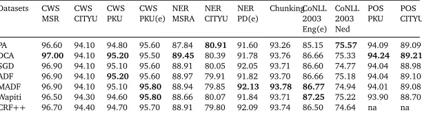
For Chinese word segmentation, we evaluate F-score using the script for SigHan 2005 bakeoff. For all NER and chunking tasks, we report phrase based F-score with the script provided by CoNLL. For POS tagging, we report token based accuracy. Results are listed in Table 5.

Datasets CWS

MSR CWSCITYU CWSPKU CWSPKU(e) NERMSRA NERCITYU NERPD(e) ChunkingCoNLL2003 Eng(e)

CoNLL 2003 Ned

POS PKU CITYUPOS

PA 96.60 94.10 94.80 95.60 87.84 80.91 91.60 93.26 85.15 75.57 94.09 89.09 DCA 97.00 94.10 95.20 95.50 89.45 80.39 91.78 93.76 86.66 75.33 94.24 89.21

SGD 96.90 94.10 95.10 95.60 88.91 80.05 92.05 93.71 86.60 74.77 94.04 88.98 ADF 96.90 94.10 95.20 95.60 88.97 79.91 91.82 93.70 86.66 75.18 94.04 89.10 MADF 96.90 94.10 95.10 95.80 88.94 79.85 92.13 93.78 86.77 74.94 94.01 89.08 Wapiti 96.50 94.30 94.60 95.80 88.66 80.07 91.84 93.71 87.25 75.22 93.90 88.70 CRF++ 96.70 94.40 94.70 95.70 88.91 79.80 92.09 93.74 86.50 74.64 na na

Table 5: Results on all datasets. Note that PA and Wapiti have different model/regularizer from other CRFs models, hence not directly comparable to other CRFs-based models. (e) means extended feature set.

3.4 Discussion

Differences across datasets: For well resourced tasks, i.e. CWS pku(e), NER People Daily(e), CoNLL 2003 English NER(e) (4,7,9 in figure 1), SGD and its variants give better performance than PA and DCA, with faster convergence speed; while PA and DCA give very robust per-formance on under-resourced tasks despite the presence of only simple token based features, partly attribute to their weight averaging mechanism. Another observation is that small or under-resourced datasets often make the learning curve of SGD and its variants fluctuate a lot. For simple datasets with only token based features, e.g. 6,10,11,12, PA and DCA performs relatively good or even better than other methods. PA is a margin based method and may generalize well to unseen data under such circumstances. Moreover, PA and DCA all use weight averaging for better generalization, which proves useful under simple feature set. In other cases, DCA performs as good as other training methods and converges as fast as SGD, but are always more stable. This may ease the selection of stopping criterion, as a non-stable learning curve may stop accidentally at a bad point. (Lavergne et al., 2010) suggest it is good practice to use a separate development set to determine a stop criterion, but this set is not always available. Note also that the aggressiveness parameterCfor PA is critical for a reasonably good performance, as in chunking (8) and English NER (9) tasks, PA gets very poor results.

0 5 10 15 20 25

4,5,6,7,9,10, the initial estimations ofη0in MADF are several times larger than that in SGD, which explains the convergence speed differences. (note the feature frequency in table 4 and convergence speed difference of SGD and MADF in figure 1.) In datasets with feature frequency not so skewed, SGD converges as fast as ADF and MADF.

ADF and MADF always converge faster than plain SGD and often achieve top performance within 10 iterations. ADF is more stable than MADF because of its fast decay of learning rate. But this effect comes at the price that ADF cannot reach top performance on some datasets. For instance, in the CWS PKU (4), Chinese NER People Daily (7) and English NER tasks (9), ADF reaches an F-score 0.1% to 0.3% lower than MADF; SGD can also performs better than ADF on these datasets after 100 iterations which I do not plot. But this is not without exception, in CoNLL 2003 Dutch NER task, where I use simple context token based features, ADF performs better than other methods. This dataset is small compared with others. The result implies ADF is more stable and suitable in most situations. MADF suffers from fluctuation on small datasets, but is still more stable, better, and faster than SGD on most datasets.

Running time: All online algorithms are 5-30 times faster than CRF++to achieve comparable performance. ADF and MADF typically need a mere 10 iterations, and other online methods need several dozens iterations to get competitive result. In terms of one pass time over the dataset, PA clearly outperforms others because it does not have to compute normalization factor and expensivelog/expoperations; DCA is only a little slower than SGD; ADF and MADF run as fast as SGD, while give more stable learning curve and faster convergence.

Batch vs. online: We plot the results of CRF++and Wapiti, which can be seen as the near optimal solution to the optimization problem, we can see online methods provide as good as or even better performance than batch method. The elastic net regularizer of Wapiti is very competitive compared withL2regularizer. Except on CoNLL 2003 English NER data, in which Wapiti exceedsL2regularizer by a large margin, they gives similar results on all datasets. Batch learning method (i.e. CRF++) rarely gives the best generalization performance. This implies that expensive batch optimization methods are not necessary for large learning tasks. Online methods will suffice. One exception is CITYU CWS task, in which CRF++performs better than all online methods. We find the problem is how a feature fires when it is false. Both CRF++and Wapiti treat it as a feature “F” and we omit it when we fire this feature. After adding this the F-score on testset goes up from 94.1% to 94.4% for SGD and MADF, 95.5% for ADF, comparable to CRF++. However, on a different dataset CWS PKU, adding this “F” feature decreases F-score by 0.1%, still higher than CRF++by 0.3%.

Summary: PA is competitive with properly chosen aggressiveness parameter on under-resourced tasks. DCA converges as fast as SGD and is more stable, and is often as good as or even better than SGD variants. ADF and MADF are consistently faster than plain SGD and often reach reasonably good performance after a mere 10 passes over the datasets. ADF sometimes gets suboptimal results and losses the opportunity to further refine the parameters because of a too fast decay of learning rate; while MADF has convergence guarantee but may have a little more fluctuation in small datasets. Finally, online methods are generally several dozens times faster and get better performance than batch method.

4 Related Work

can affect speed of SGD algorithms, resulting in a conservative small initial guess of learning rate, which slows down the convergence speed. (Sun et al., 2012) utilize feature frequency information to speed up training of CRF model. It is simple and fast compared with other Hessian approximation methods. The sparse distribution can greatly accelerate training speed of models through clever regularization as described in (Vishwanathan et al., 2006) (Bordes et al., 2009), or through sparse forward-backward decoding (Lavergne et al., 2010). Stochastic gradient descent (SGD) is well known for its performance on machine learning tasks (Bottou and Bousquet, 2008). Its recent successes in learning CRFs (Vishwanathan et al., 2006) and SVM (Shalev-Shwartz et al., 2007) show its advantage over batch learning algorithms in both convergence speed and generalization performance. It is particularly suitable in a large scale setting, and may achieve top performance even before seeing the whole dataset. Various methods based on SGD have been proposed to accelerate training of CRFs. Several variants of SGD aim at theoretically one pass over the training data to get optimal performance (Hsu et al., 2009). The core idea of these methods is approximating the inverse of Hessian in order to accelerate training (and is why they are called second order SGD). However, the approximation is expensive and much slower than a plain SGD in terms of per iteration running time. (Xu, 2011) proposes averaged SGD (ASGD) that is as fast as SGD and converges within several iterations. However, in several datasets we tested, the testset performance is below standard SGD even after we tried several switch time of SGD and ASGD.

Besides the regularizer mentioned above, group Lasso has recently been proposed to regularize a structured classifier (Martins et al., 2011). The author encodes prior structural knowledge of the feature space by grouping different features intoMgroups and using separate regularizer weight for each group. The resulting model is compact and avoids the problem of overfitting with large number of free parameters.

Conclusion

We investigate several online learning algorithms for sequence labeling and empirically show how each algorithm performs on datasets with distinct feature design and label set. This will ease the selection of algorithms in similar tasks in future. Our experiments show that most online algorithms outperform batch method (CRF++) at both speed and generalization performance. We can gain further speedup by adopting simple strategy as ADF and MADF do. We propose our own algorithm inspired by ADF, which is a variant of SGD. We confirm the effectiveness of ADF on several datasets. While ADF works in most situations, sometimes it leads to suboptimal solutions. Our algorithm performs consistently better than SGD, and converges as fast as ADF. These simple frequency adaptive methods can greatly accelerate training speed under skewed feature frequency distribution. As many NLP tasks involve the cycle of training the model and refining features then retraining the model, fast training methods are particularly useful, especially on large dataset with a large label set. It is also interesting to see how these two simple frequency adaptive approaches help in other structured learning problems in future.

Acknowledgments

References

Bordes, A., Bottou, L., and Gallinari, P. (2009). Sgd-qn: Careful quasi-newton stochastic gradient descent.The Journal of Machine Learning Research, 10:1737–1754.

Bottou, L. and Bousquet, O. (2008). The tradeoffs of large scale learning.Advances in neural information processing systems, 20:161–168.

Collins, M. (2002). Discriminative training methods for hidden markov models: Theory and experiments with perceptron algorithms. InProceedings of the 2002 Conference on Empirical Methods in Natural Language Processing, pages 1–8. Association for Computational Linguistics.

Crammer, K., Dekel, O., Keshet, J., Shalev-Shwartz, S., and Singer, Y. (2006). Online passive-aggressive algorithms.The Journal of Machine Learning Research, 7:551–585.

Hsu, C., Huang, H., Chang, Y., and Lee, Y. (2009). Periodic step-size adaptation in second-order gradient descent for single-pass on-line structured learning.Machine learning, 77(2):195–224.

Lafferty, J., McCallum, A., and Pereira, F. (2001). Conditional random fields: Probabilistic models for segmenting and labeling sequence data.

Lavergne, T., Cappé, O., and Yvon, F. (2010). Practical very large scale crfs. InProceedings of the 48th Annual Meeting of the Association for Computational Linguistics, pages 504–513, Uppsala, Sweden. Association for Computational Linguistics.

LeCun, Y., Bottou, L., Orr, G., and Müller, K. (1998). Efficient backprop. Neural networks: Tricks of the trade, pages 546–546.

Malouf, R. et al. (2002). A comparison of algorithms for maximum entropy parameter estimation. InProceedings of the sixth conference on natural language learning (CoNLL-2002), pages 49–55.

Martins, A., Gimpel, K., Smith, N., Xing, E., Figueiredo, M., and Aguiar, P. (2010). Learning structured classifiers with dual coordinate ascent. Technical report, DTIC Document.

Martins, A., Smith, N., Figueiredo, M., and Aguiar, P. (2011). Structured sparsity in structured prediction. InProceedings of the 2011 Conference on Empirical Methods in Natural Language Processing, pages 1500–1511, Edinburgh, Scotland, UK. Association for Computational Lin-guistics.

Mohit, B., Schneider, N., Bhowmick, R., Oflazer, K., and Smith, N. A. (2012). Recall-oriented learning of named entities in arabic wikipedia. InProceedings of the 13th Conference of the European Chapter of the Association for Computational Linguistics, pages 162–173, Avignon, France. Association for Computational Linguistics.

Murata, N. (1998). A statistical study of on-line learning.Online Learning and Neural Networks. Cambridge University Press, Cambridge, UK.

Nadeau, D. and Sekine, S. (2007). A survey of named entity recognition and classification.

Poon, H. and Vanderwende, L. (2010). Joint inference for knowledge extraction from biomed-ical literature. InHuman Language Technologies: The 2010 Annual Conference of the North American Chapter of the Association for Computational Linguistics, pages 813–821, Los Angeles, California. Association for Computational Linguistics.

Rabiner, L. (1989). A tutorial on hidden markov models and selected applications in speech recognition.Proceedings of the IEEE, 77(2):257–286.

Ratinov, L. and Roth, D. (2009). Design challenges and misconceptions in named entity recognition. InProceedings of the Thirteenth Conference on Computational Natural Language Learning (CoNLL-2009), pages 147–155, Boulder, Colorado. Association for Computational Linguistics.

Sha, F. and Pereira, F. (2003). Shallow parsing with conditional random fields. InProceedings of the 2003 Conference of the North American Chapter of the Association for Computational Linguistics on Human Language Technology-Volume 1, pages 134–141.

Shalev-Shwartz, S., Singer, Y., and Srebro, N. (2007). Pegasos: Primal estimated sub-gradient solver for svm. InProceedings of the 24th international conference on Machine learning, pages 807–814. ACM.

Smith, N. (2011). Linguistic structure prediction. Synthesis Lectures on Human Language Technologies, 4(2):1–274.

Song, H.-J., Son, J.-W., Noh, T.-G., Park, S.-B., and Lee, S.-J. (2012). A cost sensitive part-of-speech tagging: Differentiating serious errors from minor errors. InProceedings of the 50th Annual Meeting of the Association for Computational Linguistics (Volume 1: Long Papers), pages 1025–1034, Jeju Island, Korea. Association for Computational Linguistics.

Sun, W. and Uszkoreit, H. (2012). Capturing paradigmatic and syntagmatic lexical relations: Towards accurate chinese part-of-speech tagging. InProceedings of the 50th Annual Meeting of the Association for Computational Linguistics (Volume 1: Long Papers), Jeju Island, Korea. Sun, W. and Xu, J. (2011). Enhancing chinese word segmentation using unlabeled data. In

Proceedings of the 2011 Conference on Empirical Methods in Natural Language Processing, pages 970–979, Edinburgh, Scotland, UK. Association for Computational Linguistics.

Sun, X., Wang, H., and Li, W. (2012). Fast online training with frequency-adaptive learning rates for chinese word segmentation and new word detection. InProceedings of the 50th Annual Meeting of the Association for Computational Linguistics (Volume 1: Long Papers), pages 253–262, Jeju Island, Korea. Association for Computational Linguistics.

Tsochantaridis, I., Joachims, T., Hofmann, T., and Altun, Y. (2006). Large margin methods for structured and interdependent output variables. Journal of Machine Learning Research, 6(2):1453.

Vishwanathan, S., Schraudolph, N., Schmidt, M., and Murphy, K. (2006). Accelerated training of conditional random fields with stochastic gradient methods. InProceedings of the 23rd international conference on Machine learning, pages 969–976. ACM.