Combining Heterogeneous User Generated Data to Sense Well being

Combining Heterogeneous User Generated Data to Sense Well-being

University of Warwick Coventry, UK

[email protected]

Maria Liakata

University of Warwick Coventry, UK [email protected]

Theo Damoulas

University of Warwick Coventry, UK [email protected]

Brigitte Jellinek

Salzburg University of Applied Sciences FH Salzburg, Puch Urstein ¨Osterreich [email protected]

Weisi Guo

University of Warwick Coventry, UK [email protected]

Alexandra I. Cristea

University of Warwick Coventry, UK

[email protected]

Abstract

In this paper we address a new problem of predicting affect and well-being scales in a real-world setting of heterogeneous, longitudinal and non-synchronous textual as well as non-linguistic data that can be harvested from on-line media and mobile phones. We describe the method for collect-ing the heterogeneous longitudinal data, how features are extracted to address misscollect-ing informa-tion and differences in temporal alignment, and how the latter are combined to yield promising predictions of affect and well-being on the basis of widely used psychological scales. We achieve a coefficient of determination (R2_{) of0.71−0.76and aρof0.68−0.87which is higher than}

the state-of-the art in equivalent multi-modal tasks for affect. 1 Introduction

The World Health Organisation describes mental health as “the foundation for well-being and effective functioning for an individual and for a community” and highlights the importance of selecting suitable indicators of mental health (Herrman et al., 2005). One can distinguish between macro-level indicators, which are meant to provide a picture of generic well-being across a large population, usually at national scale, and individual indicators of mental health. Most of the macro measures typically use statistics from census, administrative and economic sources to measure the social and economic macro-environment as important determinants of mental health (e.g. Human Development Index, Gender Development Index, Human Poverty Indices (OECD, 2013). With the advent of widely available social media data, there have also been efforts to automatically obtain macro indicators of well-being and happiness, primarily through the analysis of geolocated Twitter posts (Dodds et al., 2011; Lansdall-Welfare et al., 2012; Lampos et al., 2013). These pieces of work seek to identify occurrence patterns for words with pre-defined affect scores at different levels of temporal granularity. Such approaches, with more sophisticated components for emotion recognition in social media content, can be alternatives to public surveys for mood and happiness indicators.

At the other end of the spectrum we have individual indicators of mental health. These include mea-sures of positive mental health, such as coherence & meaning in life, self-esteem etc. as well as indicators of mental distress, such as negativity, anxiety, depression (Herrman et al., 2005). These measures can be used by experts or individuals for diagnostic and management purposes, but also in aggregation, for large scale surveys. However, the reliance on self-reporting required to obtain these measures is time consum-ing and expensive and can only produce sparse data on small populations. Moreover, self-reportconsum-ing is likely to introduce bias into results. Recent work (Rachuri et al., 2010; Lathia et al., 2012; Canzian and Musolesi, 2015; Pejovic et al., 2015) shows the potential of experience sampling using mobile devices

This work is licensed under a Creative Commons Attribution 4.0 International Licence. Licence details: http://creativecommons.org/licenses/by/4.0/

for behavioural studies and clinical care, especially relating to mental health. A variety of longitudinal sensor data from a smart phone as well as location information, obtained passively from the user’s phone, can be calibrated against the user’s responses to behaviour or emotion related questions. The latter are usually harvested through regular prompts for input provided by a smart phone application.

Here we combine heterogeneous and asynchronous textual as well as non-linguistic data to train pre-dictors of well-being scores that will circumvent the need for user input. Our contributions include:

• A novel and unique dataset of heterogeneous sourcesconsisting of textual data from social media posts (Twitter, Facebook), SMS messages (>100,000), 2436 mood forms as well as asynchronous mobile phone use data including location, Wi-Fi connection, mobile phone use and sensor data (42 GB).

• Methodology for handling heterogeneous, incomplete and asynchronous data for longitudinal predictions. We consider a number of baselines and appropriate normalisations as well as an ap-proach based on multi-kernel learning, which aims to maximise the joint predictive power of each data source, and show very promising results.

• Calibration of well-being predictors based on well established affect and well-being scales, namely the Warwick-Edinburgh Mental Well-Being Scale (WEMWBS) (Tennant et al., 2007) and the Positive and Negative Affect Scale (PANAS) (Watson and Clark, 1988; Crawford and Henry, 2004).

While studies on macro-indicators have exploited simple textual features, we are not aware of another study which has worked on such an heterogeneous dataset for the automatic prediction of individual well-being scores, basing predictions on well established psychometric scales. Indeed to the best of our knowledge this is the first study to tackle predictions from heterogeneous, asynchrounous, longitudinal user generated content.

2 Related Work

et al., 2015). On the contrary, in late fusion approaches different models are trained per modality and their outputs are combined at a later stage, usually by employing weighted sum (Dobriˇsek et al., 2013; Poria et al., 2016). Gupta et al (2014) train separate classifiers on audio and video for a particular time frame and then fuse the results together to create new meta-features, while a product rule combination method is introduced for the emotion recognition task by (Dobriˇsek et al., 2013). Late fusion approaches suffer from inability to capture across-modality dependencies and thus are in contrast to our objective of combining heterogeneous data.

3 A Dataset of Heterogeneous Textual and Mobile phone data

Dataset Design: In designing our dataset we wanted to collect real-world user-generated content that could provide information about the spatio-temporal influence on users’ mental well-being. For this purpose, our goal was to combine longitudinal textual sources, such as messages and social media posts, with behavioural data, as manifested by mobility patterns and mobile phone usage. To control for the effect of variable age and stage of life we recruited student participants from the same university in a large cosmopolitan city (New York); unlike (Wang et al., 2015) the study was not confined to a campus environment. A cohort of 29 students gave us access to their Twitter and Facebook posts, SMS and Facebook messages as well as their mobile phone use data, together with location information and mobile phone sensors, over a period of 4 months each. Data collection was passive, with the exception of on-line submission of psychological tests for well-being (WEMWBS)(Tennant et al., 2007) and affect (PANAS)(Watson and Clark, 1988; Crawford and Henry, 2004), which students were asked to complete once a day, in the evening. WEMWBS was chosen as a robust, widely used measure of well-being, suitable for the general population and employed by the NHS. Since WEMWBS focusses on positive attributes, we also used PANAS to capture negative emotions. Unlike other work, we did not require any other manual effort from students such as the completion of on-line questionnaires mapping them to personality traits or prompts for self-reported emotional status.

Data Collection: The data was primarily collected from the Twitter API and two applications (Apps) that were installed for the purpose of the study, on the participants’ mobile phones. The first App is DeviceAnalyzer (Wagner et al., 2013), which collects a wide range of time-stamped data, including location and phone usage (e.g. number and duration of calls). SMS data was collected through the NUS SMS collection App1_{, which was configured to retrieve a batch of SMS messages authorised by}

a participant, as a weekly email. Users were asked to complete psychological scales (mood forms) by logging into a secure webserver, set up for the study. We collected a total of 2436 mood forms, each corresponding to completed PANAS and WEMWBS scales. Facebook data was downloaded by our participants twice during their time on the study and was uploaded to the secure webserver, where the participants could choose the data they wished to share and make available to us. We thus collected 111,270 textual posts and 42GB of DA data spanning the period February 2015-December 2015. Note that participants’ time on the study was staggered, with each participant contributing data for 4 months. Dataset Description: The data is heterogeneous by nature and design and asynchronous, with variable temporal granularity, reflecting a real-world scenario and presenting numerous challenges. The most challenges are presented by the DeviceAnalyzer (DA) data, due to their sheer volume and natural redun-dancy. For example, aggregates are required to represent most DA features (e.g. number of calls, time spent in a location etc.) but choosing the best aggregate and its respective temporal granularity is not straightforward. Moreover, timestamps are presented in epochs, so they had to be converted to absolute values, to be in alignment with those of textual data. We experimented with different methods for aggre-gation; for the purpose of this study, the decision was made to aggregate DA features at the hour level, by taking mean or cumulative values for the feature within an hourly interval. We selected a subset (153) of the DA features that can be potentially indicative of user behaviour, as opposed to being related to purely technical aspects of the phone. The former, among others, include: volume of images and SMS messages, physical sensor readings (physical environment and movement), location in terms of

tude and latitude as well as wireless network and data transfer (digital environment), battery level, ringer and other phone settings (user choices). Data is collected anonymously and linked together through user identifiers.

Location and Wi-Fi connection data:A further challenge was presented by how to make use of location and Wi-Fi connection data to allow: (a) compatibility with numeric aggregates (b) direct comparisons between different users, who inevitably spend time at different locations with different Wi-Fi connec-tions, with no direct semantic mappings. Our solution to the above was to rank locations and Wi-Fi connections, respectively, according to the time spent in each of them, by each user. Thus we collected the top 10 locations and Wi-Fi connections per user. See also section 4.2.

Sensor data: There are 15 different sensors of which only accelerometer and light sensor data are provided by 22 of the 29 participants. Each of the two sensors corresponds to 10 different values, including resolution and range of values at a particular time-point.

Textual data:The fields associated with each textual instance are the speaker, the raw text, the absolute time stamp, the data source (e.g. Facebook) and the type of text (e.g. message).

Mood forms: Obtaining scores for the mood forms is straightforward and based on the scoring instruc-tions associated with each of the two psychological scales.

4 Methodology

4.1 Data matrix creation and Features

Our goal here is to combine features from both (i) the DeviceAnalyzer (DA) data and (ii) the textual sources (TEXT), in order to train a model that can automatically predict mood scores originating from the three daily mood forms. The latter correspond to the determination of positive affect (“positive”) and negative affect (“negative”), calculated on the basis of the PANAS psychological scale and well-being (“wellwell-being”), calculated on the basis of the WEMWBS psychological scale. Those three scores for positive, negative and well-being constitute our target values. Past research has shown a strong correlation between being and positive (r=.71) and a moderate (negative) correlation between well-being and negative affect (r=-.54) (Tennant et al., 2007). For the purpose of this work we keep the three targets distinct from each other, to aid the interpretability of results.

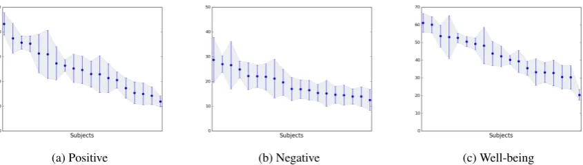
We had 29 participants on the study who agreed to give us access to both their DA and TEXT data and complete daily mood forms. During the study, two participants switched to iPhones, so they could no longer run DA on their mobile phones. For others, there was missing DA data, where missing data are defined as cases where one or more sources of DA data have no values for longer than a 6 hour period before the completion of a mood form, which was assumed as being most relevant for its completion. TEXT data on the other hand are never considered missing, as the lack of a post is considered to be a choice and a useful indicator of user behaviour. For the purposes of the current paper, we focused thus on the 19 users for whom we had both DA and TEXT data and no missing data in the 6 hour period prior to the completion of a mood form. This means that from an original set of 2436 mood forms, each corresponding to three mood score values, several textual posts (Twitter, Facebook, SMS) and several GB of DA data, we make use of 1438 mood forms and the corresponding features and target values.Thus, for this study, we used 40,786 textual posts written in English and the corresponding DA data (∼10GB). Mood scores consist in scores for well-being, positive and negative affect. Figure 1 shows the mean values and the standard deviations for the three mood form scores based on the subjects that were used in our study. The average per-subject score is 25.2,19.2 and42.6 for the positive, negative and well-being target respectively. Interestingly, we observe that the average per-subject standard deviation is5.0,

4.9and5.7 for the three targets, pointing to the subjects’ affect and well-being fluctuations during the studied period, which makes our task more challenging and shows that simply identifying a subject based on his/her id is not sufficient for predicting his/her mood.

(a) Positive (b) Negative (c) Well-being

Figure 1: Average and standard deviations of the mood form scores obtained by the 19 subjects.

underlying assumption is that those features generated by a user during the past day are most likely to have influenced her mood, resulting in the observed mood scores. Thus, given a mood form completed by a certain user at timet, we focused on her past24hours beforet, in order to extract our features from and aggregate these features in different time windows within the 24 hour period, and, more specifically, into 5 different windows (1, 6, 12, 18 and 24 hours before the completion of a mood form), to allow for an extra level of granularity to the effect of proximity to the mood form timestamp. This process was performed for the DA features that are described in the following section and not for the TEXT ones, which are only considered at the 24 hour window. This is due to the sparsity of some feature representations of the latter. In future work, we plan to make better use of the temporal granularity of the TEXT features and their interaction with the DA data. In the following, we describe a number of baselines, utilising subsets of the features (4.2) and different algorithms, tested under different settings (4.3) to establish the most effective approach to combining heterogeneous data for prediction.

4.2 Baseline definition Baseline DA Features

Previous work in a controlled user study (Wang and Harari, 2015) looked at exploiting features from students’ mobile phone usage within a semester, to predict student academic performance at the end of the semester. While we consider target objectives at much finer grained temporal intervals, we adopt a baseline from mobile phone data (DA) to approximate the ones considered in the StudentLife study (Wang et al., 2015). The latter relies on pre-built classifiers (i.e., accelerometer data (Lu et al., 2010)) to make use of sensor data, such as accelerometer, while we use aggregates of raw data. In our work, we have built classifiers that take into account all data variables, and as such offer more degrees of freedom, to better understand the underlying causes of emotions than studies that consist of disparate pre-built classifiers. Our DA baseline consists of:

• Calls: The total number and duration of the calls that a subject has made and received. • Locations: The percentage of time that a subject has spent in herith_{preferred location.}

• Wi-Fi:: The percentage of time that a subject has spent while connected to herith_{preferred Wi-Fi.}

• Other: the percentage of time that a user’s mobile: (i) headphones have been “on” (“off”); (ii) screen brightness has been set to “manual” (“auto”); (iii) airplane mode has been “active” (“inac-tive”); (iv) ringer mode has been set to “vibrate”, “silent” and “normal”; (v) headset has been “on” (“off”); and (vi) has been disconnected, plugged in a USB port and plugged in AC.

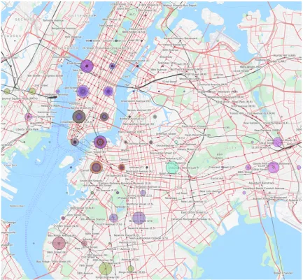
Figure 2: Geo-visual projection of the subjects’ visited locations. Each colour indicates a unique user and the size of their spot indicates the number of unique GPS samples at that location.

five different time windows, before the completion of a mood form (1,6,12,18and24hours), leading to 200 DA features per instance. In the case of missing data for some feature (e.g. missing locations due to disconnections), we filled-in the gaps, by replacing the missing values of a feature with the past 6-hour mean of the same feature for that specific user. For example, if we have no indication of the time spent in particular locations 1 hour prior to the completion of a mood form, we use the 6-hour mean of each location feature from the 6-hour window leading up to the timestamp of the mood form for the user in question. If after this process an instance would still have some missing feature values, we would drop the instance out of our analysis. This resulted in reducing our dataset from2436instances (mood forms completed by 29 users) to1,438complete ones, corresponding to 19 different users. Note that while we have sensor data from the phones (accelerometer and light sensor), and accelerometer data were quite predictive in the StudentLife study, we have not used them for the purposes of the current study, due to a large number of missing values exceeding a 6-hour window.

Baseline TEXT Features

All the texts (SMS and social media posts/messages) sent by a specific user over the past24hours before the completion of a mood form were concatenated in one 24-hour window. Focusing only on the English texts2_{, the following commonly applied practices were performed: lowercasing, tokenisation (Gimpel et}

al., 2011), replacement of usernames and URLs with placeholders, “usrmnt” and “urlink”, respectively. We extracted the following textual features as potentially relevant to the mental state of users:

• Ngrams: We extractedtfidf representations of uni- and bi-grams, setting the max (min) document frequency to 99% (1%) and excluding all English stopwords, for noise reduction purposes.

• Word embeddings: We used the word embeddings created by (Tang et al., 2014), which have been used successfully before for the task of sentiment analysis, related to our problem. The unigrams of every text were matched against those vectors and seven functions were applied on every dimension of the resulting matrix (mean, median, min, max, stdev, first and third quartile).

• Lexicons: We employed several lexicons that have been effectively used in sentiment- or emotion-related works. Those were the Opinion Lexicon (Hu and Liu, 2004), NRC Hashtag, NRC Hashtag Emotion (Mohammad, 2012), Unigram and Bigram NRC Hashtag Sentiment and Sentiment 140 lexicons (Zhu et al., 2014), MaxDiff Twitter Sentiment Lexicon (Svetlana Kiritchenko and Moham-mad, 2014), MSOL (Mohammad et al., 2009) and AFINN (Nielsen, 2011). For lexicons providing binary values (pos/neg), we counted the number of ngrams matching each of the positive and nega-tive classes; for those lexicons with score values, we used the simple counts and the total summation of the corresponding scores from each ngram in the text matched against the lexicons.

• Topics: In order to better categorise the content that a subject has shared and to accommodate the sparse representations of the ngrams, we used the word clusters created by Preot¸iuc-Pietro et al. (2015), which were based on word2vec representations of the most common keywords appearing on Twitter over a 2-month period. We measured the cosine similarity of the unigrams of every textual instance with each one of the200word clusters.

• Other: We extracted the following features related to the social activity level of a user: the number of SMS messages, Facebook posts, Facebook messages, Facebook images, twitter posts, twitter messages, and the total number of tokens and textual items (messages or posts) in the instance. 4.3 Experiments and Models

We applied five regression models, in order to predict each of the three target mood scores separately. All models were tested using 5-fold cross validation using the two sets of features (DA, TEXT) individually and in combination (ALL). Before feeding our features to the regression models, various transformations and normalisation techniques were tested. Those include:

• The root transformation of the target labels, often used in regression models to inflate the differ-ence between lower values and stabilise the differdiffer-ence between higher scores3_.

• Combinations of: (a) normalisation(linear transformation of feature values to the [−1,1] range, based on the maximum/minimum value of the feature),(b) standardisation(zero mean, unit vari-ance) or(c) no transformation.

Those transformations were performed on (i) a per-user basis (so that the feature values of different users become more comparable) and (ii) an overall basis (as a final transformation of all features from different users before applying our models). Notice that in the case of the per-user transformations, the model suffers from the cold-start problem, as it expects to have some past knowledge about the user, in order to predict her mood.

The algorithms that were tested under this setup were Linear Regression, LASSO, Random Forest for regression (RF), Support Vector Regression (SVR) and a multi-kernel SVR approach. The first four algorithms were chosen as widely accepted standards for regression problems, as well as for their diver-sity (two linear models, one with and one without feature selection, an ensemble of trees, a kernel-based method). Multi-kernel learning (MKL) was proposed in order to allow for a more advanced handling of the different data sources, by jointly learning different kernels, each optimised to a particular data source. For LASSO, different experiments with respect to the alpha parameter were tested (10−2_{, ...,10}2_{); for}

RF we set the number of estimators to200, after experimentation; for SVR we have used the Gaussian Kernel with varying kernel width and C values (all combinations of{10−2_{, ...,10}2_{}for both)}4_.

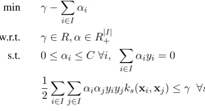
One drawback of SVR is the difficulty to interpret predictions and feature importance. Similarly per-forming algorithms, such as RF, can provide some indication of feature importance in the model learnt, but, when dealing with heterogeneous data sources, data source contribution is a lot less straightforward. For these reasons, we applied an MKL approach (Sonnenburg et al., 2006), which jointly learns an op-timal combination of source-specific kernels. Formally, for a training set comprised of instancesI and featuresS partitioned in subgroupss ∈ S, we apply a base kernelk per feature subgroup with some weightw, as follows: f(x) =P_i∈IαiPs∈Swsks(x,xi) +bwhere the parametersαi, the bias termb

and the kernel weights are estimated by solving the optimisation problem:

min γ−X

i∈I

αi

w.r.t. γ ∈R, α∈R|₊I| s.t. 0≤αi ≤C∀i,

X

i∈I

αiyi = 0

1 2

X

i∈I

X

j∈I

αiαjyiyjks(xi,xj)≤γ ∀s

We have opted for theL2norm to regularise the kernel weights. In order to compare our MKL approach

with SVR, we selected one Gaussian kernel per feature set (9 kernels: 4 DA and 5 TEXT, for each of the feature sources defined in 4.2) and tuned the width of every kernel and the C parameter performing the same grid search as with SVR. This implies that we have used the same width for all nine kernels in every run. Further kernel selection and parameter optimisation techniques could be used, but those are out of the scope of the current work.

5 Evaluation and Results

We have used two standard measures for evaluating our models – the root mean squared error (RMSE, ) and the coefficient of determination (R2_{) . Those were selected in order to compare both the errors}

between the different approaches as well as the proportion of the variance that is predictable by them. Table 1 presents the results obtained from our models. We provide separate results of the models for the two cases with respect to the per-user transformation of the features. Only the best transformation combinations are presented per model and the results obtained by Linear Regression are omitted, due to its poor performance. The feature transformation that was used is provided as an index.

In terms of comparing the three tasks (predicting each of the targets), our models can successfully capture much of the target variance in their predictions with respect to the well-being target. The lowest errors are observed with respect to the negative target (the comparison with the well-being case in terms of the error is not straight-forward, due to the larger scale that is used in WEMWBS). However,R2_for

this task is considerably lower, pointing to the low variance in each model’s prediction.

The task of user normalisation does not appear to have any significant effect when applied on the DA features for any task, implying that our models trained on DA features are user-independent and can generalise well. However, this is not the case for the TEXT features: for all algorithms and all tasks, the performance drops significantly when no user normalisation is applied. This is an interesting finding, pointing to future work on text-based user modelling, as it provides some evidence that population-wide analyses on mood prediction tasks that do not take it into account can be ineffective.

The comparison between the different algorithms illustrates that RF is the best in most experiments with respect to all target scores, achieving anR2 _{of.76in the best case (predicting the well-being score}

Positive Negative Well-being

+User Norm –User Norm +User Norm –User Norm +User Norm –User Norm

R2 _R2 _R2 _R2 _R2 _R2

D

A

LASSO n,n.31 8.24 s.35 7.99 n,n.11 6.71 s.22 6.25 n,n.30 10.51 s.35 10.15

RF s,s.69 5.55 s.64 5.95 s,s.43 5.38 −.40 5.49 s,s.75 6.33 s.67 7.18

SVR n,n.58 6.38 n.60 6.27 n,n.35 5.74 n.36 5.69 n,n.62 7.80 n.62 7.77

MKL n,n.61 6.15 −.59 6.36 n,n.38 5.60 n.33 5.82 n,s.65 7.43 n.62 7.80

TEXT

LASSO n,n.53 6.80 n.06 9.59 n,n.23 6.23 n.02 7.02 n,n.55 8.46 n.10 11.96

RF −,s.70 5.42 n.13 9.22 −,s.45 5.26 n.07 6.85 s,s.74 6.36 s.21 11.19

SVR n,n.60 6.27 n.11 9.31 n,n.32 5.87 n.06 6.88 n,n.62 7.72 n.19 11.30

MKL n,n.62 6.08 n.14 9.16 n,n.36 5.69 −.06 6.89 n,n.65 7.43 n.22 11.12

ALL

LASSO n,n.49 7.07 n.31 8.20 n,n.18 6.41 n.20 6.33 n,n.54 8.52 n.38 9.92

RF −,s.71 5.31 n.63 6.00 −,s.46 5.20 s.40 5.51 n,s.76 6.23 −.68 7.12 SVR n,n.60 6.27 n.55 6.62 n,n.34 5.76 n.31 5.88 n,n.62 7.75 n.58 8.17

MKL n,n.65 5.84 n.61 6.14 n,n.41 5.45 n.36 5.67 n,n.68 7.12 n.64 7.58

Table 1: R2 _{root mean squared error () of the different models based on the three feature sets (DA,}

TEXT, ALL) and with respect to the three different ground truth scores (positive, negative, well-being). Values for both setups with respect to the user normalisation (with and without) are presented. The index used in theR2 _{column indicates the (i) final and (ii) per-user normalisation of the best-performing}

setup (nfor normalisation,sfor standardisation,−for none). Only the final normalisation method (i) is indicated in experiments performed without per-user normalisation.

(a) Positive (b) Negative (c) Well-being

Figure 3: Actual VS Predicted charts for the best performing algorithm (RF) on the three targets.

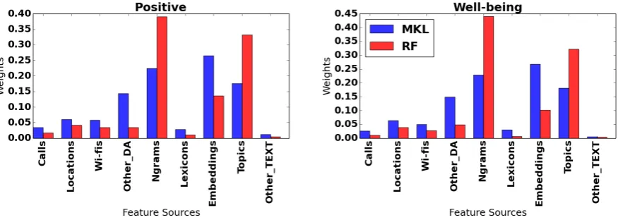
Figure 4: Feature set weights in RF (red) and MKL (blue) for the positive and the well-being targets, training on all features in the per-user normalisation approach.

other hand, it also explains the difference in accuracy between the two models, which can be highly re-duced with further tuning of the MKL kernels and their parameters. Importantly though, the comparison between the feature weights of the two algorithms also explains the relatively small boost in accuracy that RF achieves when the DA features are incorporated in the TEXT-based RF (see Table 1), since the algorithm is relying much more on the TEXT features (12.7%, 18.0% and 12.7% of the feature weights come from DA sources with respect to positive, negative and well-being, compared to 29.5%, 28.9% and 28.7% for MKL). This means that MKL has much more potential in making use of heterogeneous sources compared to RF and further tuning of our MKL approach can provide an even more balanced kernel weighting for robustness purposes, while also increasing performance.

6 Conclusion and Future Work

We have presented a new real-world dataset consisting of heterogeneous, longitudinal and asynchronous textual and mobile phone use data. We have investigated different approaches for combining this hetero-geneous data for daily predictions of mood scores and have proposed some strong baselines as well as a multi-kernel learning approach that learns a combination of source-specific representations, giving very promising results. We achieve a coefficient of determination (R2_{) of0.71−0.76and aρof0.68−0.87}

which is higher than the state-of-the art in equivalent multi-modal tasks for affect.

In the future we aim to address the following: (a) optimise our MKL component and make better use of temporal granularity, by means of convolution and spectral mixture kernels (Lukasik and Cohn, 2016; Wilson et al., 2014) (b) look into the semantics of different locations and (c) address the challenge of missing data in one type of source, which is currently resulting in the loss of a large number of instances. Finally, we plan to apply our micro-level text-based model presented in this paper to the macro-level. Most approaches on predicting population-wide well-being indices based on online media have primarily relied on lists of pre-defined keywords, without using a per-user ground truth and ignoring the user modelling aspect. By applying our model on such a data stream, we will investigate whether we can build effective macro-level indicators for monitoring the well-being of a large population.

Acknowledgements

References

Mohammad Akbari, Liqiang Nie, and Tat-Seng Chua. 2015. amm: Towards adaptive ranking of multi-modal documents. International Journal of Multimedia Information Retrieval, 4(4):233–245.

Andrey Bogomolov, Bruno Lepri, and Fabio Pianesi. 2013. Happiness recognition from mobile phone data. In

Social Computing (SocialCom), 2013 International Conference on, pages 790–795. IEEE.

Andrey Bogomolov, Bruno Lepri, Michela Ferron, Fabio Pianesi, and Alex Sandy Pentland. 2014. Daily stress recognition from mobile phone data, weather conditions and individual traits. InProceedings of the 22nd ACM

international conference on Multimedia, pages 477–486. ACM.

L. Canzian and M. Musolesi. 2015. Trajectories of Depression: Unobtrusive Monitoring of Depressive States by means of Smartphone Mobility Traces Analysis. InACM Ubicomp.

J. Crawford and J. Henry. 2004. The Positive and Negative Affect Schedule (PANAS): Construct validity, mea-surement properties and normative data in a large non-clinical sample. British Journal of Clinical Psychology, 43.

Simon Dobriˇsek, Rok Gajˇsek, France Miheliˇc, Nikola Paveˇsi´c, and Vitomir ˇStruc. 2013. Towards efficient multi-modal emotion recognition.Int J Adv Robotic Sy, 10(53).

Peter Sheridan Dodds, Kameron Decker Harris, Isabel M. Kloumann, Catherine A. Bliss, and Christopher M. Danforth. 2011. Temporal patterns of happiness and information in a global social network: Hedonometrics and twitter. PLoS ONE, 6(12):e26752, 12.

Kevin Gimpel, Nathan Schneider, Brendan O’Connor, Dipanjan Das, Daniel Mills, Jacob Eisenstein, Michael Heilman, Dani Yogatama, Jeffrey Flanigan, and Noah A Smith. 2011. Part-of-speech tagging for twitter: Annotation, features, and experiments. InProceedings of the 49th Annual Meeting of the Association for

Com-putational Linguistics: Human Language Technologies: short papers-Volume 2, pages 42–47. Association for

Computational Linguistics.

Rahul Gupta, Nikolaos Malandrakis, Bo Xiao, Tanaya Guha, Maarten Van Segbroeck, Matthew Black, Alexandros Potamianos, and Shrikanth Narayanan. 2014. Multimodal prediction of affective dimensions and depression in human-computer interactions. InProceedings of the 4th International Workshop on Audio/Visual Emotion

Challenge, pages 33–40. ACM.

Helen Herrman, Shekhar Saxena, Rob Moodie, et al. 2005. Promoting mental health: concepts, emerging evi-dence, practice: a report of the World Health Organization, Department of Mental Health and Substance Abuse

in collaboration with the Victorian Health Promotion Foundation and the University of Melbourne. World

Health Organization.

Minqing Hu and Bing Liu. 2004. Mining and summarizing customer reviews. InProceedings of the tenth ACM

SIGKDD international conference on Knowledge discovery and data mining, pages 168–177. ACM.

Natasha Jaques, Sara Taylor, Akane Sano, and Rosalind Picard. 2015. Multi-task, multi-kernel learning for estimating individual wellbeing. InProc. NIPS Workshop on Multimodal Machine Learning, Montreal, Quebec. V. Lampos, T. Welfare, R. Araya, and N. Christianini. 2013. Analysing Mood Patterns in the United Kingdom

through Twitter Content. arXiv: 1304.5507v.

Thomas Lansdall-Welfare, Vasileios Lampos, and Nello Cristianini. 2012. Nowcasting the mood of the nation. Significance, 9(4):26–28.

N. Lathia, D. Quercia, and J. Crowcroft. 2012. The Hidden Image of the City: Sensing Community Well-Being from Urban Mobility. Pervasive Computing, 7319.

Hong Lu, Jun Yang, Zhigang Liu, Nicholas D. Lane, Tanzeem Choudhury, and Andrew T. Campbell. 2010. The jigsaw continuous sensing engine for mobile phone applications. InACM Conference on Embedded Networked Sensor Systems (SenSys 2010).

Michal Lukasik and Trevor Cohn. 2016. Convolution kernels for discriminative learning from streaming text. In Thirtieth AAAI Conference on Artificial Intelligence. Citeseer.

Saif Mohammad, Cody Dunne, and Bonnie Dorr. 2009. Generating high-coverage semantic orientation lexicons from overtly marked words and a thesaurus. InProceedings of the 2009 Conference on Empirical Methods in

Saif Mohammad. 2012. #emotional tweets. In*SEM 2012: The First Joint Conference on Lexical and Computa-tional Semantics – Volume 1: Proceedings of the main conference and the shared task, and Volume 2:

Proceed-ings of the Sixth International Workshop on Semantic Evaluation (SemEval 2012), pages 246–255, Montr´eal,

Canada, 7-8 June. Association for Computational Linguistics.

Finn ˚Arup Nielsen. 2011. A new anew: Evaluation of a word list for sentiment analysis in microblogs. arXiv preprint arXiv:1103.2903.

OECD. 2013. Hows life? 2013: Measuring well-being.

Veljko Pejovic, Neal Lathia, Cecilia Mascolo, and Mirco Musolesi. 2015. Mobile-based experience sampling for behaviour research.arXiv preprint arXiv:1508.03725.

Soujanya Poria, Erik Cambria, Amir Hussain, and Guang-Bin Huang. 2015. Towards an intelligent framework for multimodal affective data analysis. Neural Networks, 63:104–116.

Soujanya Poria, Erik Cambria, Newton Howard, Guang-Bin Huang, and Amir Hussain. 2016. Fusing audio, visual and textual clues for sentiment analysis from multimodal content. Neurocomputing, 174:50–59.

Daniel Preot¸iuc-Pietro, Svitlana Volkova, Vasileios Lampos, Yoram Bachrach, and Nikolaos Aletras. 2015. Study-ing user income through language, behaviour and affect in social media. PloS one, 10(9):e0138717.

K. Rachuri, M. Musolesi, C. Mascolo, P. Renfrow, C. Longworth, and A. Aucinas. 2010. EmotionSense: A Mobile Phones based Adaptive Platform for Experimental Social Psychology Research. InACM Ubicomp. S¨oren Sonnenburg, Gunnar R¨atsch, Christin Sch¨afer, and Bernhard Sch¨olkopf. 2006. Large scale multiple kernel

learning.Journal of Machine Learning Research, 7(Jul):1531–1565.

Xiaodan Zhu Svetlana Kiritchenko and Saif M. Mohammad. 2014. Sentiment analysis of short informal texts. 50:723–762.

Duyu Tang, Furu Wei, Nan Yang, Ming Zhou, Ting Liu, and Bing Qin. 2014. Learning sentiment-specific word embedding for twitter sentiment classification. InACL (1), pages 1555–1565.

R. Tennant, L. Hiller, R. Fishwick, S. Platt, S. Joseph, S. Weich, J. Parkinson, J. Secker, and S. Stewart-Brown. 2007. The Warwick-Edinburgh Mental Well-being Scale (WEMWBS):development and UK validation. Health and Quality of Life Outcomes, 5.

D. Wagner, A. Rice, and A. Beresford. 2013. Device Analyzer: Understanding smartphone usage. InInternational

Conference on Mobile and Ubiquitous Systems: Computing, Networking and Services.

R. Wang and G. Harari. 2015. SmartGPA: How Smartphones Can Assess and Predict Academic Performance of College Students. InACM Ubicomp.

Min Wang, Donglin Cao, Lingxiao Li, Shaozi Li, and Rongrong Ji. 2014. Microblog sentiment analysis based on cross-media bag-of-words model. InProceedings of international conference on internet multimedia computing

and service, page 76. ACM.

R. Wang, F. Chen, Z. Chen, T. Li, G. Harari, S. Tignor, X. Zhou, D. Ben-Zeev, and A. Campbell. 2015. Stu-dentLife: Assessing Mental Health, Academic Performance and Behavioral Trends o College Students using Smartphones. InACM Ubicomp.

D. Watson and L. Clark. 1988. Development and Validation of Brief Measures of Positive and Negative Affect: The PANAS Scales.Journal of Personality and Social Psychology, 54.

Andrew Wilson, Elad Gilboa, John P Cunningham, and Arye Nehorai. 2014. Fast kernel learning for multidimen-sional pattern extrapolation. InAdvances in Neural Information Processing Systems, pages 3626–3634. Matthias Wimmer, Bj¨orn Schuller, Dejan Arsic, Gerhard Rigoll, and Bernd Radig. 2008. Low-level fusion of

audio, video feature for multi-modal emotion recognition. InVISAPP (2), pages 145–151.