Experiments in Idiom Recognition
Jing Peng and Anna Feldman
Department of Computer Science Department of Linguistics Montclair State University Montclair, New Jersey, USA 07043
Abstract
Some expressions can be ambiguous between idiomatic and literal interpretations depending on the context they occur in, e.g.,saleshit the roof vs. hit the roofof the car. We present a novel method of classifying whether a given instance is literal or idiomatic, focusing on verb-noun constructions. We report state-of-the-art results on this task using an approach based on the hypothesis that the distributions of the contexts of the idiomatic phrases will be different from the contexts of the literal usages. We measure contexts by using projections of the words into vector space. For comparison, we implement Fazly et al. (2009)’s, Sporleder and Li (2009)’s, and Li and Sporleder (2010b)’s methods and apply them to our data. We provide experimental results validating the proposed techniques.
1 Introduction
Researchers have been investigating idioms and their properties for many years. According to traditional approaches, an idiom is — in its simplest form— a string of two or more words for which meaning is not derived from the meanings of the individual words comprising that string (Swinney and Cutler, 1979). As such, the meaning ofkick the bucket(‘die’) cannot be obtained by breaking down the idiom and an-alyzing the meanings of its constituent parts, to kick and the bucket. In addition to being influenced by the principle of compositionality, the traditional approaches are also influenced by theories of generative grammar (Flores, 1993; Langlotz, 2006) The properties that traditional approaches attribute to idiomatic expressions are also the properties that make them difficult for generative grammars to describe. For instance, idioms can be syntactically ill-formed (e.g.,by and large), resistant to grammatical transfor-mations (e.g.,the bucket was kicked by him6=‘die’), impervious to lexical substitutions (e.g.,kick the pail6=‘die’), and semantically ambiguous without context. This last property of the idioms is what we address in our work. The examples below illustrate the ambiguity1.
(A1) After the last page was sent to the printer, an editor wouldring a bell, walk toward the door, and holler ” Good night! ” (Literal)
(A2) His name never fails toring a bellamong local voters. Nearly 40 years ago, Carthan was elected mayor of Tchula. . . (Idiomatic)
(B1) . . . that caused the reactor to literallyblow its top. About 50 tons of nuclear fuel evaporated in the explosion. . . (Literal)
(B2) . . . He didn’t pound the table, he didn’tblow his top. He always kept his composure. (Idiomatic) (C1) . . . coming out of the fourth turn, slid down the track,hitthe insidewalland then hit the attenuator at the start of pit road. (Literal)
(C2) . . . job training, research and more havehita Republicanwall. (Idiomatic)
Fazly et al. (2009)’s analysis of 60 idioms from the British National Corpus (BNC) has shown that close to half of these also have a clear literal meaning; and of those with a literal meaning, on average This work is licensed under a Creative Commons Attribution 4.0 International Licence. Licence details: http://creativecommons.org/licenses/by/4.0/
1These examples are extracted from the Corpus of Contemporary American English (COCA) (http://corpus.byu.
edu/coca/)
around 40% of their usages are literal.
Just to motivate our work, idioms present great challenges for many Natural Language Processing (NLP) applications. Current machine translation systems (MT), unfortunately, more frequently than not, are not able to translate idiomatic expressions correctly.
Here’s an example how the English utteranceHe didn’t pound the table, he didn’tblow his top. He always kept his composure. is translated by Bing and Google Translate from English into Russian and Chinese.
(1) a. English original: He didn’t pound the table, he didn’t blow his top. He always kept his composure.
b. Bing: Chinese: 他没拍几下桌子,他并没有打打打击击击他他他的的的上上上方方方。他总是保持镇静。 c. Google: Chinese: 他没有拍桌子,他没有吹吹吹他他的他的的上上上面面面。他始终保持着镇定。
d. Bing: Russian: Он не фунт за столом, он не взорвать его сверху. Он всегда держал его спокойствие.
e. Google:Russian: Он не фунт стол, он не взрывал его вершину. Он всегда держал его хладнокровие.
In all the examples above, blow his top is translated as ‘destruction/explosion of his top/summit’, which is clearly not the intended meaning.
In this paper we describe an algorithm for automatic classification of idiomatic and literal expressions. Similar to Peng et al. (2014), we treat idioms as semantic outliers. Our assumption is that the context word distribution for a literal expression will be different from the distribution for an idiomatic one. We capture the distribution in terms of covariance matrix in vector space.
2 Proposed Techniques
We build our work on the following hypotheses:
1. Words representing local topics are likely to associate strongly with a literal expression appearing in that text segment;
2. The context word distribution for a literal expression in word vector space is different from the distribution of an idiomatic one. (This hypothesis is central to the distributional approach to meaning (Firth, 1957; Katz and Giesbrecht, 2006).)
2.1 Projection Based On Local Context Representation
The local context of a literal target verb-noun construction (VNC) must be different from that of an idiomatic one. We propose to exploit recent advances in vector space representation to capture the difference between local contexts (Mikolov et al., 2013a; Mikolov et al., 2013b).
A word can be represented by a vector of fixed dimensionality q that best predicts its surrounding words in a sentence or a document (Mikolov et al., 2013a; Mikolov et al., 2013b). Given such a vector representation, our first proposal is the following. Letvandnbe the vectors corresponding to the verb and noun in a target verb-noun construction, as in blow whistle, where v ∈ <q represents blow and n ∈ <q representswhistle. Letσvn = v+n ∈ <q. Thus,σvn is the word vector that represents the composition of verbvand nounn, and in our example, the composition ofblowandwhistle. As indicated in Mikolov et al. (2013b), word vectors obtained from deep learning neural net models exhibit linguistic regularities, such as additive compositionality. Therefore,σvn is justified to predict surrounding words of the composition of, say,blowandwhistlein the literal usage ofblow whistle. Our hypothesis is that on average, inner productσblowwhistle·v, wherevs are context words in a literal usage, should be greater thanσblowwhistle·v, wherevs are context words in an idiomatic usage.
our notation, we have thatσblowwhistle =vblow+vwhistle. It follows thatp=σblowwhistle·vrepresents the inner product ofσblowwhistle and a context wordv. The following table shows the inner products of σblowwhistle and context wordsvin the two sentences, after removing functional words. From the above
Table 1: Inner products withσblowwhistle are you going whole lot mean university people well -0.13 0.28 0.20 -0.03 0.04 0.00 -0.17 -0.14 -0.05
start timed run students ran hard they could 0.15 0.12 0.19 -0.22 0.14 0.15 -0.02 0.04
table,σBlowW histle has a larger inner product value (0.069) with context words in the literal usage than with context words in the idiomatic usage (0.000), on average.
For a given vocabulary ofmwords, represented by matrixV = [v1, v2,· · ·, vm]∈ <q×m, we calculate the projection of each wordviin the vocabulary ontoσvn
P =Vtσvn (1)
whereP ∈ <m, andtrepresents transpose. Here we assume thatσvn is normalized to have unit length. Thus,Pi =vt
iσvnindicates how strongly word vectorviis associated withσvn. This projection, or inner product, forms the basis for our proposed technique.
LetD = {d1, d2,· · ·, dl}be a set ofltext segments (local contexts), each containing a target VNC (i.e.,σvn). Instead of generating a term by document matrix, where each term istf ·idf (product of term frequency and inverse document frequency), we compute a term by document matrixMD ∈ <m×l, where each term in the matrix is
p·idf, (2)
the product of the projection of a word onto a target VNC and inverse document frequency. That is, the term frequency (tf) of a word is replaced by the projection (inner product) of the word ontoσvn(1). Note that if segmentdj does not contain wordvi,MD(i, j) = 0, which is similar totf·idf estimation. The motivation is that topical words are more likely to be well predicted by a literal VNC than by an idiomatic one. The assumption is that a word vector is learned in such a way that it best predicts its surrounding words in a sentence or a document (Mikolov et al., 2013a; Mikolov et al., 2013b). As a result, the words associated with a literal target will have larger projection onto a target σvn. On the other hand, the projections of words associated with an idiomatic target VNC ontoσvn should have a smaller value. We also propose a variant ofp·idf representation. In this representation, each term is a product ofpand typicaltf ·idf. That is,
p·tf·idf. (3)
2.2 Local Context Distributions
Our second hypothesis states that words in a local context of a literal expression will have a different dis-tribution from those in the context of an idiomatic one. We propose to capture local context disdis-tributions in terms of scatter matrices in a space spanned by word vectors (Mikolov et al., 2013a; Mikolov et al., 2013b).
Letd= (w1, w2· · ·, wk)∈ <q×kbe a segment (document) ofkwords, wherewi ∈ <qare represented by a vectors (Mikolov et al., 2013a; Mikolov et al., 2013b). Assumingwis have been centered without loss of generality, we compute the scatter matrix
Σ =dtd, (4)
whereΣrepresents the local context distribution for a given target VNC.
(Fukunaga, 1990). Both measures require the knowledge of matrix determinant. In our case, this can be problematic, becauseΣ(4) is most likely to be singular, which would result in a determinant to be zero. We propose to measure the difference betweenΣ1andΣ2using matrix norms. We have experimented with the Frobenius norm and the spectral norm. The Frobenius norm evaluates the difference betweenΣ1 andΣ2when they act on a standard basis. The spectral norm, on the other hand, evaluates the difference when they act on the direction of maximal variance over the whole space.
3 Experiments 3.1 Methods
We have carried out an empirical study evaluating the performance of the proposed techniques. For comparison, the following methods are evaluated.
1. tf·idf: compute term by document matrix from training data withtf·idf weighting.
2. p·idf: compute term by document matrix from training data with proposedp·idf weighting (2). 3. p·tf·idf: compute term by document matrix from training data with proposedp·tf·idf weighting
(3).
4. CoVARFro: proposed technique (4) described in Section 2.2, the distance between two matrices is computed using Frobenius norm.
5. CoVARSp: proposed technique similar toCoVARFro. However, the distance between two matrices is determined using the spectral norm.
6. Context+ (CTX+): supervised version of the CONTEXT technique described in Fazly et al. (2009) (see below).
7. TextSim: supervised classification using the Dice coefficient (see below).
8. GMM: Gaussian Mixture Model as described in Li and Sporleder (2010b) (see below).
For methods from1to3, we compute a latent space from a term by document matrix obtained from the training data that captures 80% variance. To classify a test example, we compute cosine similarity between the test example and the training data in the latent space to make a decision.
For methods4and5, we compute literal and idiomatic scatter matrices from training data (4). For a test example, we compute a scatter matrix according to (4), and calculate the distance between the test scatter matrix and training scatter matrices using the Frobenius norm for method4, and the spectral norm for method5.
Method6corresponds to a supervised version of CONTEXT described in (Fazly et al., 2009). CON-TEXT is unsupervised because it does not rely on manually annotated training data, rather it uses knowl-edge about automatically acquired canonical forms (C-forms). C-forms are fixed forms corresponding to the syntactic patterns in which the idiom normally occurs. Thus, the gold-standard is “noisy” in CONTEXT. Here we provide manually annotated training data. That is, the gold-standard is “clean.” Therefore, CONTEXT+ is a supervised version of CONTEXT. We implemented this approach from scratch since we had no access to the code and the tools used in the original article and applied this method to our dataset and the performance results are reported in Table 3.
Method 7 corresponds to a supervised classifier described in Sporleder and Li (2009). In the ex-periments described in Sporleder and Li (2009), this method achieved the best performance. We used the Dice coeffiient as implemented in Ted Pedersen’s Text::Similarity module (http://www.d.umn. edu/œtpederse/text-similarity.htmlto determine the word overlap of a test instance with the literal and non-literal instances in the training set (for the same expression) and then assign the label of the closest set. A similar approach has been described in Katz and Giesbrecht (2006).
comparing which Gaussian has the higher probability of generating a specific instance. While the original Li and Sporleder (2010b)’s work uses Normalized Google Distance to model semantic relatedness in computing features (Cilibrasi and Vit´anyi, 2007; Cilibrasi and Vit´anyi, 2009), we use inner product between word vectors as described in section 3.3. The main reason is that Google’s custom search engine API is no longer free. The detection task is done by a Bayes decision rule, which chooses the category by maximizing the probability of fitting the data into different Gaussian components: c(x) = arg maxi∈{l,n}{wi ×N(x|µi,Σi)}, wherecis the category of the Gaussian,µi is the mean,Σi is the covariance matrix, andwiis the mixture weight.
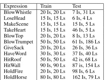
Table 2: Datasets: Is = idioms; Ls = literals Expression Train Test
BlowWhistle 20 Is, 20 Ls 7 Is, 31 Ls LoseHead 15 Is, 15 Ls 6 Is, 4 Ls MakeScene 15 Is, 15 Ls 15 Is, 5 Ls TakeHeart 15 Is, 15 Ls 46 Is, 5 Ls BlowTop 20 Is, 20 Ls 8 Is, 13 Ls BlowTrumpet 50 Is, 50 Ls 61 Is, 186 Ls GiveSack 20 Is, 20 Ls 26 Is, 36 Ls HaveWord 30 Is, 30 Ls 37 Is, 40 Ls HitRoof 50 Is, 50 Ls 42 is, 68 Ls HitWall 90 Is, 90 Ls 87 is, 154 Ls HoldFire 20 Is, 20 Ls 98 Is, 6 Ls HoldHorse 80 Is, 80 Ls 162 Is, 79 Ls
3.2 Data Preprocessing
We use BNC (Burnard, 2000) and a list of verb-noun constructions (VNCs) extracted from BNC by Fazly et al. (2009) and Cook et al. (2008) and labeled as L (Literal), I (Idioms), or Q (Unknown). The list contains only those VNCs whose frequency was greater than 20 and that occurred at least in one of two idiom dictionaries (Cowie et al., 1983; Seaton and Macaulay, 2002). The dataset consists of 2,984 VNC tokens. For our experiments we only use VNCs that are annotated as I or L. We only experimented with idioms that can have both literal and idiomatic interpretations. We should mention that our approach can be applied to any syntactic construction. We decided to use VNCs only because this dataset was available and for fair comparison – most work on idiom recognition relies on this dataset.
We use the original SGML annotation to extract paragraphs from BNC. Each document contains three paragraphs: a paragraph with a target VNC, the preceding paragraph and following one. Our data is summarized in Table 2.
Since BNC did not contain enough examples, we extracted additional ones from COCA, COHA and GloWbE (http://corpus.byu.edu/). Two human annotators labeled this new dataset for idioms and literals. The inter-annotator agreement was relatively low (Cohen’s kappa = .58); therefore, we merged the results keeping only those entries on which the two annotators agreed.
3.3 Word Vectors
For our experiments reported here, we obtained word vectors using the word2vec tool (Mikolov et al., 2013a; Mikolov et al., 2013b) and the text8 corpus. The text8 corpus has more than 17 million words, which can be obtained from mattmahoney.net/dc/text8.zip. The resulting vocabulary has 71,290 words, each of which is represented by aq = 200dimension vector. Thus, this 200 dimensional vector space provides a basis for our experiments.
3.4 Datasets
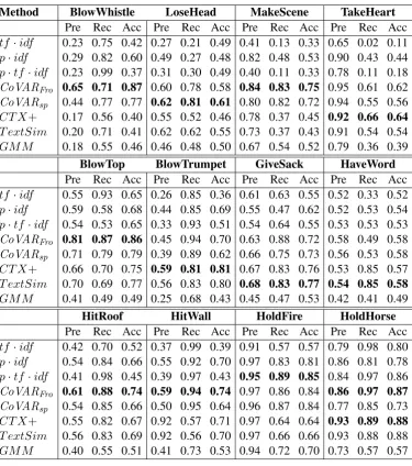
Table 3: Average accuracy of competing methods on 12 datasets
Method BlowWhistle LoseHead MakeScene TakeHeart Pre Rec Acc Pre Rec Acc Pre Rec Acc Pre Rec Acc tf ·idf 0.23 0.75 0.42 0.27 0.21 0.49 0.41 0.13 0.33 0.65 0.02 0.11 p·idf 0.29 0.82 0.60 0.49 0.27 0.48 0.82 0.48 0.53 0.90 0.43 0.44 p·tf ·idf 0.23 0.99 0.37 0.31 0.30 0.49 0.40 0.11 0.33 0.78 0.11 0.18 CoVARFro 0.65 0.71 0.87 0.60 0.78 0.58 0.84 0.83 0.75 0.95 0.61 0.62 CoVARsp 0.44 0.77 0.77 0.62 0.81 0.61 0.80 0.82 0.72 0.94 0.55 0.56 CT X+ 0.17 0.56 0.40 0.55 0.52 0.46 0.78 0.37 0.45 0.92 0.66 0.64 T extSim 0.20 0.71 0.41 0.62 0.62 0.55 0.73 0.37 0.43 0.91 0.54 0.54 GMM 0.18 0.55 0.46 0.46 0.48 0.50 0.67 0.54 0.52 0.79 0.36 0.39
BlowTop BlowTrumpet GiveSack HaveWord Pre Rec Acc Pre Rec Acc Pre Rec Acc Pre Rec Acc tf ·idf 0.55 0.93 0.65 0.26 0.85 0.36 0.61 0.63 0.55 0.52 0.33 0.52 p·idf 0.59 0.58 0.68 0.44 0.85 0.69 0.55 0.47 0.62 0.52 0.53 0.54 p·tf ·idf 0.54 0.53 0.65 0.33 0.93 0.51 0.54 0.64 0.55 0.53 0.53 0.53 CoVARFro 0.81 0.87 0.86 0.45 0.94 0.70 0.63 0.88 0.72 0.58 0.49 0.58 CoVARsp 0.71 0.79 0.79 0.39 0.89 0.62 0.66 0.75 0.73 0.56 0.53 0.58 CT X+ 0.66 0.70 0.75 0.59 0.81 0.81 0.67 0.83 0.76 0.53 0.85 0.57 T extSim 0.70 0.69 0.77 0.56 0.83 0.80 0.68 0.83 0.77 0.54 0.85 0.58 GMM 0.41 0.49 0.49 0.25 0.68 0.43 0.45 0.47 0.53 0.42 0.41 0.49
HitRoof HitWall HoldFire HoldHorse
Pre Rec Acc Pre Rec Acc Pre Rec Acc Pre Rec Acc tf ·idf 0.42 0.70 0.52 0.37 0.99 0.39 0.91 0.57 0.57 0.79 0.98 0.80 p·idf 0.54 0.84 0.66 0.55 0.92 0.70 0.97 0.83 0.81 0.86 0.81 0.78 p·tf ·idf 0.41 0.98 0.45 0.39 0.97 0.43 0.95 0.89 0.85 0.84 0.97 0.86 CoVARFro 0.61 0.88 0.74 0.59 0.94 0.74 0.97 0.86 0.84 0.86 0.97 0.87 CoVARsp 0.54 0.85 0.66 0.50 0.95 0.64 0.96 0.87 0.84 0.77 0.85 0.73 CT X+ 0.55 0.82 0.67 0.92 0.57 0.71 0.97 0.64 0.64 0.93 0.89 0.88 T extSim 0.56 0.83 0.69 0.92 0.56 0.70 0.97 0.66 0.66 0.93 0.88 0.88 GMM 0.40 0.55 0.51 0.41 0.73 0.53 0.94 0.72 0.70 0.73 0.57 0.57
BlowWhistle:we can immediately turn towards a high-pitched sound such as whistle being blown. The ability to accurately locate a noise· · ·LoseHead: This looks as eye-like to the predator as the real eye and gives the prey a fifty-fifty chance of losing its head. That was a very nice bull I shot, but I lost his head. MakeScene: · · ·in which the many episodes of life were originally isolated and there was no relationship between the parts, but at last we must make a unified scene of our whole life. TakeHeart:
· · ·cutting off one of the forelegs at the shoulder so the heart can be taken out still pumping and offered to the god on a plate.BlowTop:Yellowstone has no large sources of water to create the amount of steam to blow its top as in previous eruptions.
4 Results
Table 4: Performance results by class: I denotes the idiom class and L denotes the literal class. Method tf·idf p·idf p·tf·idf CoVarFro CoVarSP CT X+ T extSim GMM
Is Ls Is Ls Is Ls Is Ls Is Ls Is Ls Is Ls Is Ls BlowWhistle 0.75 0.35 0.82 0.55 0.99 0.23 0.71 0.90 0.77 0.76 0.56 0.37 0.71 0.34 0.55 0.44 LoseHead 0.21 0.92 0.27 0.80 0.30 0.79 0.78 0.27 0.81 0.30 0.52 0.36 0.62 0.43 0.48 0.53 MakeScene 0.13 0.92 0.48 0.70 0.11 0.97 0.83 0.51 0.82 0.40 0.37 0.68 0.37 0.59 0.54 0.46 TakeHeart 0.02 0.93 0.43 0.56 0.11 0.80 0.61 0.69 0.55 0.62 0.66 0.42 0.54 0.50 0.36 0.67 BlowTop 0.93 0.48 0.58 0.74 0.53 0.72 0.87 0.86 0.79 0.79 0.70 0.77 0.69 0.82 0.49 0.49 BlowTrumpet 0.85 0.20 0.85 0.64 0.93 0.38 0.94 0.62 0.89 0.54 0.81 0.81 0.83 0.79 0.68 0.35 GiveSack 0.63 0.49 0.47 0.72 0.64 0.49 0.88 0.61 0.75 0.71 0.83 0.71 0.83 0.72 0.47 0.57 HaveWord 0.33 0.70 0.53 0.56 0.53 0.54 0.49 0.66 0.53 0.62 0.85 0.31 0.85 0.32 0.41 0.56 HitRoof 0.70 0.40 0.84 0.56 0.98 0.12 0.88 0.65 0.85 0.53 0.82 0.58 0.83 0.60 0.55 0.49 HitWall 0.99 0.05 0.92 0.57 0.97 0.12 0.94 0.63 0.95 0.47 0.57 0.78 0.56 0.92 0.73 0.42 HoldFire 0.57 0.46 0.83 0.50 0.89 0.26 0.86 0.54 0.87 0.48 0.64 0.66 0.66 0.72 0.72 0.37 HoldHorse 0.98 0.45 0.81 0.72 0.97 0.63 0.97 0.67 0.85 0.49 0.89 0.86 0.88 0.87 0.57 0.57 Average 0.59 0.53 0.65 0.64 0.66 0.50 0.81 0.64 0.79 0.56 0.68 0.61 0.70 0.64 0.55 0.49
Interestingly, the Frobenius norm outperforms the spectral norm. One possible explanation is that the spectral norm evaluates the difference when two matrices act on the maximal variance direction, while the Frobenius norm evaluates on a standard basis. That is, Frobenius measures the difference along all basis vectors. On the other hand, the spectral norm evaluates changes in a particular direction. When the difference is a result of all basis directions, the Frobenius norm potentially provides a better measurement. The projection methods (p·idf andp·tf ·idf) outperformtf ·idf overall but not as pronounced asCoVAR.
tf.idf p.idf p.tf.idf CoVARFroCoVARsp CT X+ T extSim GM M 0
0.1 0.2 0.3 0.4 0.5 0.6 0.7 0.8 0.9
Precision Recall Accuracy
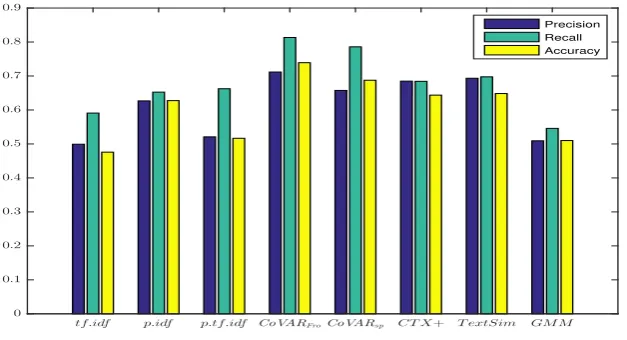
Figure 1: Aggregated performance by the eight competing methods on the 12 data sets.
Finally, we have noticed that even the best model (CoVARFro) does not perform as well on certain idiomatic expressions. We hypothesize that the model works the best on highly idiomatic expressions. to be more easily interpretable than others.
scores, such as 2 vs. 3. The annotators tried to avoid ranking the expressions as 100% idiomatic or 100% literal. Measuring the agreement using ranges is reasonable. Thus, if both annotators marked an idiom as 1 or 2, we considered them to be in agreement. The ranges were 1-2, 2-3, 3-4 and 4-5. Applying this method, the annotator agreement increased significantly – 80% (Cohen’s Kappa 0.68).
The table shows that the low ranking scores often correspond to the low performance scores of our best model: the model did not perform well onHaveWord and the idiomaticity score produced by the human annotators is relatively low (=2). Low idiomaticity suggests indeterminate contexts, which affects the performance of our context-based models. There is a positive correlation between the degree of idiomaticity and the accuracy of the best model (r=.47,p=< .001).
Table 5: Idiomaticity Rank: 1=low; 5 = high
VNC HitWall GiveSack HaveWord LoseHead MakeScene BlowTop BlowWhistle HoldFire HoldHorse HitRoof TakeHeart
Rank 1.5 2 2 2 2.5 3 3 3.5 3.5 4 4
5 Related Work
Previous approaches to idiom detection can be classified into two groups: 1) type-based extraction, i.e., detecting idioms at the type level; 2) token-based detection, i.e., detecting idioms in context. Type-based extraction is based on the idea that idiomatic expressions exhibit certain linguistic properties such as non-compositionality that can distinguish them from literal expressions (Sag et al., 2002; Fazly et al., 2009). While many idioms do have these properties, all idioms fall on the continuum from being compositional to being partly unanalyzable to completely non-compositional (Cook et al., 2007). Katz and Giesbrecht (2006), Birke and Sarkar (2006), Fazly et al. (2009), Li and Sporleder (2009), Li and Sporleder (2010a), Sporleder and Li (2009), and Li and Sporleder (2010b), among others, notice that type-based approaches do not work on expressions that can be interpreted idiomatically or literally depending on the context and thus, an approach that considers tokens in context is more appropriate for idiom recognition. To address these problems, Peng et al. (2014) investigate the bag of words topic representation and incorporate an additional hypothesis–contexts in which idioms occur are more affective. Still, they treat idioms as semantic outliers.
6 Conclusions
In this paper we described an original algorithm for automatic classification of idiomatic and literal expressions. We also compared our algorithms against several competing idiom detection algorithms in the literature. The performance results show that our algorithm generally outperforms Fazly et al. (2009)’s, Sporleder and Li (2009), and Li and Sporleder (2010b)’s models (see Table 4). In particular, our method is especially effective when idioms are highly idiomatic. A research direction is to incorprate affect into our model. Idioms are typically used to imply a certain evaluation or affective stance toward the things they denote (Nunberg et al., 1994; Sag et al., 2002). We usually do not use idioms to describe neutral situations, such as buying tickets or reading a book. Even though our method was tested on verb-noun constructions, it is independent of syntactic structure and can be applied to any idiom type. Unlike Fazly et al. (2009)’s approach, for example, our algorithm is language-independent and does not rely on POS taggers and syntactic parsers, which are often unavailable for resource-poor languages. Our next step is to expand this method and use it for idiom detection rather than for idiom classification.
Acknowledgments
References
Julia Birke and Anoop Sarkar. 2006. A clustering approach to the nearly unsupervised recognition of nonliteral language. InProceedings of the 11th Conference of the European Chapter of the Association for Computational Linguistics (EACL’06), pages 329–226, Trento, Italy.
Lou Burnard, 2000. The British National Corpus Users Reference Guide. Oxford University Computing Services. Rudi Cilibrasi and Paul M. B. Vit´anyi. 2007. The google similarity distance. IEEE Trans. Knowl. Data Eng.,
19(3):370–383.
Rudi Cilibrasi and Paul M. B. Vit´anyi. 2009. Normalized web distance and word similarity. CoRR, abs/0905.4039. Paul Cook, Afsaneh Fazly, and Suzanne Stevenson. 2007. Pulling their weight: Exploiting syntactic forms for the automatic identification of idiomatic expressions in context. InProceedings of the ACL 07 Workshop on A
Broader Perspective on Multiword Expressions, pages 41–48.
Paul Cook, Afsaneh Fazly, and Suzanne Stevenson. 2008. The VNC-Tokens Dataset. InProceedings of the LREC
Workshop: Towards a Shared Task for Multiword Expressions (MWE 2008), Marrakech, Morocco, June.
Anthony P. Cowie, Ronald Mackin, and Isabel R. McCaig. 1983. Oxford Dictionary of Current Idiomatic English, volume 2. Oxford University Press.
Afsaneh Fazly, Paul Cook, and Suzanne Stevenson. 2009. Unsupervised Type and Token Identification of Id-iomatic Expressions.Computational Linguistics, 35(1):61–103.
John R. Firth. 1957. A synopsis of linguistic theory, 1930–1955. InStudies in Linguistic Analysis, Special volume of the Philological Society, pages 1–32. Blackwell, Oxford.
d’Arcais Flores. 1993. The comprehension and semantic interpretation of idioms. Idioms: Processing, structure, and interpretation, pages 79–98.
K. Fukunaga. 1990.Introduction to statistical pattern recognition. Academic Press.
Graham Katz and Eugenie Giesbrecht. 2006. Automatic Identification of Non-compositional Multiword Ex-pressions using Latent Semantic Analysis. In Proceedings of the ACL/COLING-06 Workshop on Multiword Expressions: Identifying and Exploiting Underlying Properties, pages 12–19.
Andreas Langlotz. 2006. Idiomatic creativity: a cognitive-linguistic model of representation and idiom-variation in English, volume 17. John Benjamins Publishing.
Linlin Li and Caroline Sporleder. 2009. A cohesion graph based approach for unsupervised recognition of literal and non-literal use of multiword expresssions. InProceedings of the 2009 Workshop on Graph-based Methods
for Natural Language Processing (ACL-IJCNLP), pages 75–83, Singapore.
Linlin Li and Caroline Sporleder. 2010a. Linguistic cues for distinguishing literal and non-literal usages. In
COLING (Posters), pages 683–691.
Linlin Li and Caroline Sporleder. 2010b. Using gaussian mixture models to detect figurative language in context.
InProceedings of NAACL/HLT 2010.
Tomas Mikolov, Kai Chen, Greg Corrado, and Jeffrey Dean. 2013a. Efficient estimation of word representations in vector space. InProceedings of Workshop at ICLR.
Tomas Mikolov, Ilya Sutskever, Kai Chen, Greg Corrado, and Jeffrey Dean. 2013b. Distributed representations of words and phrases and their compositionality. InProceedings of NIPS.
Geoffrey Nunberg, Ivan A. Sag, and Thomas Wasow. 1994. Idioms. Language, 70(3):491–538.
Jing Peng, Anna Feldman, and Ekaterina Vylomova. 2014. Classifying idiomatic and literal expressions using topic models and intensity of emotions. InProceedings of the 2014 Conference on Empirical Methods in
Nat-ural Language Processing (EMNLP), pages 2019–2027, Doha, Qatar, October. Association for Computational
Linguistics.
Ivan A. Sag, Timothy Baldwin, Francis Bond, Ann Copestake, and Dan Flickinger. 2002. Multiword expressions: A Pain in the Neck for NLP. InProceedings of the 3rd International Conference on Intelligence Text Processing
Maggie Seaton and Alison Macaulay, editors. 2002. Collins COBUILD Idioms Dictionary. HarperCollins Pub-lishers, second edition.
Caroline Sporleder and Linlin Li. 2009. Unsupervised Recognition of Literal and Non-literal Use of Idiomatic Expressions. InEACL ’09: Proceedings of the 12th Conference of the European Chapter of the Association for
Computational Linguistics, pages 754–762, Morristown, NJ, USA. Association for Computational Linguistics.