Text Categorization using Feature Projections
Youngjoong Ko
Department of Computer Science, Sogang University 1 Sinsu-dong, Mapo-gu
Seoul, 121-742, Korea [email protected],
Jungyun Seo
Department of Computer Science, Sogang University 1 Sinsu-dong, Mapo-gu
Seoul, 121-742, Korea [email protected]
Abstract
This paper proposes a new approach for text categorization, based on a feature projection technique. In our approach, training data are represented as the projections of training documents on each feature. The voting for a classification is processed on the basis of individual feature projections. The final classification of test documents is determined by a majority voting from the individual classifications of each feature. Our empirical results show that the proposed approach, Text Categorization using Feature Projections (TCFP), outperforms k-NN, Rocchio, and Naïve Bayes. Most of all, TCFP is about one hundred times faster than k-NN. Since TCFP algorithm is very simple, its implementation and training process can be done very easily. For these reasons, TCFP can be a useful classifier in the areas, which need a fast and high-performance text categorization task.
Introduction
An issue of text categorization is to classify documents into a certain number of pre-defined categories. Text categorization is an active research area in information retrieval and machine learning. A wide range of supervised learning algorithms has been applied to this issue, using a training data set of categorized documents. The Naïve Bayes (McCalum et al., 1998; Ko et al., 2000), Nearest Neighbor (Yang et al., 2002), and Rocchio (Lewis et al., 1996) are well-known algorithms.
Among these learning algorithms, we focus
on the Nearest Neighbor algorithm. In particular, the k-Nearest Neighbor (k-NN) classifier in text categorization is one of the state-of-the-art methods including Support Vector Machine (SVM) and Boosting algorithms. Since the Nearest Neighbor algorithm is much simpler than the other algorithms, the k-NN classifier is intuitive and easy to understand, and it learns quickly. But the weak point of k-NN is too slow at running time. The main computation is the on-line scoring of all training documents, in order to find the k nearest neighbors of a test document. In order to reduce the scaling problem in on-line ranking, a number of techniques have been studied in the literature. Techniques such as instance pruning technique (Wilson et al., 2000) and projection (Akkus et al., 1996) are well known.
The instance pruning technique is one of the most straightforward ways to speed classification in a nearest neighbor system. It reduces time necessary and storage requirements by removing instances from the training set. A large number of such reduction techniques have been proposed, including the Condensed Nearest Neighbor Rule (Hart, 1968), IB2 and IB3 (Aha et al., 1991), and the Typical Instance Based Learning (Zhang, 1992). These and other reduction techniques were surveyed in depth in (Wilson et al., 1999), along with several new reduction techniques called DROP1-DROP5. Of these, DROP4 had the best performance.
this approach, the classification knowledge is represented as the sets of projections of training data on each feature dimension. The classification of an instance is based on a voting by the k nearest neighbors of each feature in a test instance. The resulting system allowed the classification to be much faster than that of k-NN and its performance were comparable with k-NN.
In this paper, we present a particular implementation of text categorization using feature projections. When we applied the feature projection technique to text categorization, we found several problems caused by the special properties of text categorization problem. We describe these problems in detail and propose a new approach to solve them. The proposed system shows the better performance than k-NN and it is much faster than k-NN.
The rest of this paper is organized as follows. Section 1 simply presents k-NN and k-NNFP algorithm. Section 2 explains a new approach using feature projections. In section 3, we discuss empirical results in our experiments. Section 4 is devoted to an analysis of time complexity and strong points of the new proposed classifier. The final section presents conclusions.
1. k-NN and k-NNFP Algorithm
In this section, we simply describe k-NN and k-NNFP algorithm.
1.1 k-NN Algorithm
As an instance-based classification method, k-NN has been known as an effective approach to a broad range of pattern recognition and text classification problems (Duda et al., 2001; Yang, 1994). In k-NN algorithm, a new input instance should belong to the same class as their k nearest neighbors in the training data set. After all the training data is stored in memory, a new input instance is classified with the class of k nearest neighbors among all stored training instances.
For the distance measure and the document representation, we use the conventional vector space model in text categorization; each document is represented as a vector of term
weights, and similarity between two documents is measured by the cosine value of the angle between the corresponding vectors (Yang et al., 2002).
Let a document d with n terms (t) be represented as the feature vector:
> =<w(t1,d),w(t2,d ),...,w(t ,d )
d n
r r
r r
(1)
We compute the weight vectors for each document using one of the conventional TF-IDF schemes (Salton et al., 1988). The weight of term t in document d is calculated as follows:
d
n N d
t tf d
t
w r t
r
r (1 log (, )) log( / )
) ,
( = + × (2)
where
i) w( dt,r)is the weight of term t in document dr ii) tf( dt,r)is the within-document Term Frequency (TF) iii) log(N/nt) is the Inverted Document Frequency
(IDF)
iv)N is the number of documents in the training set v) nt is the number of training documents in which t
occurs
vi)
∑
∈ =
d t wt d
dr r (,r)2 is the 2-norm of vector dr
Given an arbitrary test document d, the k-NN classifier assigns a relevance score to each candidate category cj using the following
formula:
∑
∈ ′
′ =
j
k d D
R d
j d d d
c s
I r r
r r r
) (
) , cos( )
,
( (3)
where Rk(d) r
denotes a set of the k nearest neighbors of document d and Dj is a set of
training documents in class cj.
1.2 k-Nearest Neighbor on Feature Projection (k-NNFP) Algorithm
distance between two instances di and dj with
regard to m-th feature tm is distm(tm(i), tm(j)) as
follows:
) , ( ) , ( )) ( ), (
(tm i tm j wtm di wtm dj distm
r r
−
= (4)
where tm(i)denotes m-th feature t in a instance
i
dr .
The classification on a feature is done according to votes of the k-nearest neighbors of that feature in a test instance. The final classification of the test instance is determined by a majority voting from individual classification of each feature. If there are n features, this method returns n×k votes whereas k-NN method returns k votes.
2. A New Approach of Text
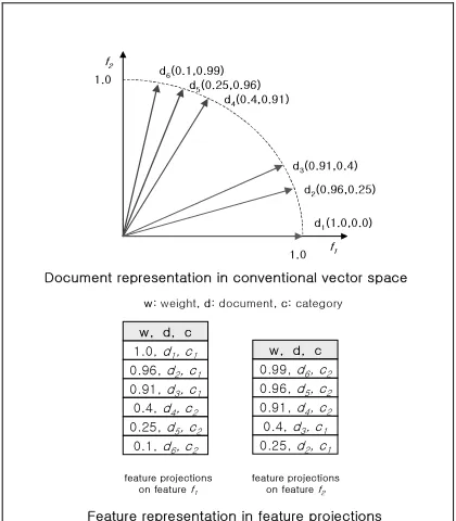
Categorization on Feature Projections First of all, we show an example of feature projections in text categorization for more easy understanding. We then enumerate the problems to be duly considered when the feature projection technique is applied to text categorization. Finally, we propose a new approach using feature projections to overcome these problems.
2.1 An Example of Feature Projections in Text Categorization
We give a simple example of the feature projections in text categorization. To simplify our description, we suppose that all documents have just two features (f1 and f2) and two
categories (c1 and c2). The TF-IDF value by
formula (2) is used as the weight of a feautre. Each document is normalized as a unit vector and each category has three instances:
{
1 2 3}
1 d ,d ,dc = and c2=
{
d4,d5,d6}
. Figure 1shows how document vectors in conventional vector space are transformed into feature projections and stored on each feature dimension. The result of feature projections on a term (or feature) can be seen as a set of weights of documents for the term. Since a term with 0.0 weight is useless, the size of the set equals to the DF value of the term.
XUW
XUW XOXUWSWUWP
YOWU`]SWUY\P
[OWU[SWU`XP
ZOWU`XSWU[P
:
;
\OWUY\SWU`]P
]OWUXSWU``P
kGGGGG kGGGGG
mGGGG mGGGG
XUWSGXSGX WU`]SGYSGX WU`XSGZSGX WU[SG[SGY WUY\SG\SGY
WUXSG]SGY WUY\SGYS X WU[SGZS X WU`XSG[S Y WU`]SG\S Y WU``SG]S Y
G
GG: GGG;
SGGSGG
SGGSGG
SGGSGG aGSGaGSGaG
Figure 1. Feature representation on feature projections
2.2 Problems in Applying Feature Projections to Text Categorization
There are three problems: (1) the diversity of the Document Frequency (DF) values of terms, (2) the property of using TF-IDF value of a term as the weight of the feature, and (3) the lack of contextual information.
2.2.1 The diversity of the Document Frequency values of terms
Table 1 shows a distribution of the DF values of the terms in Newsgroup data set. The numerical values of Table 1 are calculated from training data set with 16,000 documents and 10,000 features chosen by feature selection. The k in fourth column means the number of nearest neighbors selected in k-NNFP; the k in k-NNFP was set to 20 in our experiments.
Table 1. A distribution of the DF values of the terms in Newsgroup data set
Average DF
maximum DF
Minimum DF
The # of features DF < k (20)
According to Table 1, more than a half of the features have the DF values less than k (20). This result is also explained by Zipf’s law. The problem is that some features have the DF values less than k while other features have the DF values much greater than k. For a feature that has a DF value less than k, all the elements of the feature projections on the feature could and should participate for voting. In this case, the number of elements chosen for voting is less than k. For other features, only maximum k elements among the elements of the feature projections should be chosen for voting. Therefore, we need to normalize the voting ratio for each feature. As shown in formula (5), we use a proportional voting method to normalize the voting ratio.
2.2.2 The property of using TF-IDF value of a term as weight of a feature
The TF-IDF value of a term is their presumed value for identifying the content of a document (Salton et al., 1983). On feature projections, elements with a high TF-IDF value for a feature become more useful classification criterions for the feature than any elements with low TF-IDF values. Thus we use only elements with TF-IDF values above the average TF-IDF value for voting. The selected elements also participate for proportional voting with the same importance as TF-IDF value of each element. The voting ratio of each category cj in a feature tm(i) of a test
document di r
is calculated by the following formula:
In above formula, Imdenotes a set of elements
selected for voting and y(cj,tm(l))∈
{ }
0.1 is afunction; if the category for a element tm(l)is
equal to cj, the output value is 1. Otherwise, the
output value is 0.
2.2.3 The lack of contextual information Since each feature votes separately on feature projections, contextual information is missed. We use the idea of co-occurrence frequency for applying contextual information to our
algorithm.
To calculate a co-occurrence frequency value between two terms tiand tl, we count the number
of documents that include both terms. It is separately calculated in each category of training data. Finally, the co-occurrence frequency value of two terms is obtained by a maximum value among co-occurrence frequency values in each category as follows:
{
( , , )}
co denotes a co-occurrence frequency
value of tiand tlin a category cj.
TF-IDF values of two terms ti and tj, which
occur in a test document d, are modified by reflecting the co-occurrence frequency value. That is, the terms with a high co-occurrence frequency value and a low category frequency value could have higher term weights as follows:
where i) tw(ti,d) denotes a modified term weight
assigned to term ti, ii) cf denotes the category
frequency, the number of categories in which ti
and tj co-occur, and iii) maxco(ti,tj) is the maximum value among all co-occurrence frequency values.
Finally, in order to apply these improvements (formulae (5) and (7)) to our algorithm, we calculate the voting score of each category cj
in tmof a test document di r
as the following formula:
2.3 A New Text Categorization Algorithm using Feature Projections
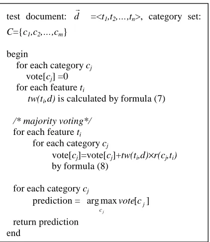
A new text categorization algorithm using feature projections, named TCFP, is described in the following:
In training phase, our algorithm needs only a very simple process; the training documents are projected on their each feature and numerical values for the proportional voting (formula (5)) are calculated.
3. Empirical Evaluation
3.1 Data Sets and Experimental Settings To test our proposed approach, we used two different data sets. For fair evaluation, we used the five-fold cross-validation method. Therefore, all results of our experiments are averages of five runs.
The Newsgroups data set, collected by Ken Lang, contains about 20,000 articles evenly divided among 20 UseNet discussion groups (McCalum et al., 1998). After removing words that occur only once or on a stop word list, the average vocabulary from five training data has 51,325 words (with no stemming). The second data set comes from the WebKB project at CMU (Yang et al., 2002). We use the four most populous entity-representing categories: course,
faculty, project, and student. The resulting data set consists of 4,198 pages with a vocabulary of 18,742 words. It is an uneven data set; the largest category has 1,641 pages and the smallest one has 503 pages.
We applied statistical feature selection at a preprocessing stage for each classifier, using a
2
χ statistics (Yang et al., 1997).
To compare TCFP to other algorithms for speeding classification, we implemented k-NNFP and k-NN with reduction. We used DROP4 as reduction technique (Wilson et al., 1999). By DROP4, only 26% of the original training documents in both data sets was retained. The k in k-NNFP was set to 20 and the k in k-NN with reduction was set to 30. In addition, we implement other classifiers: Naive Bayes, k-NN, and Rocchio classifier. The k in k-NN was set to 30 and andα=16 andβ=4 were used in Rocchio classifier.
As performance measures, we followed the standard definition of recall, precision, and F1
measure. For evaluating performance average across categories, we used the micro-averaging method.
3.2 Experimental Results
3.2.1 Comparison of TCFP and k-NN (and other algorithms for speeding classification ) Figure 2 and Table 2 show results from TCFP, k-NN, k-NN with reduction, and k-NNFP. In addition, we added other type of TCFP to our experiment. It was TCFP without contextual information (not using formula (7)).
Figure 2. Comparison of TCFP ,k-NN, k-NNFP, and
k-NN with reduction test document: dr =<t1,t2,…,tn>, category set:
C={c1,c2,…,cm}
begin
for each categorycj
vote[cj] =0
for each featureti
tw(ti,d) is calculated by formula (7)
/* majority voting*/
for each featureti
for each categorycj
vote[cj]=vote[cj]+tw(ti,d)×r(cj,ti)
by formula (8)
for each categorycj
prediction = argmax [ j]
c
c vote
j
Table 2. The top micro-average F1of each classifier
TCFP
TCFP without context
k-NN k-NNFP
k-NN
with reduction
85.41 85.14 85.15 81.93 81.34
As a result, TCFP achieved the highest micro-average F1 score. Also, TCFP without
contextual information presented the nearly same performance as k-NN. Although, over all vocabulary sizes, TCFP without contextual information achieved little lower performance than TCFP, it also can be useful classifier for its simplicity and the fast running time(see Table 5).
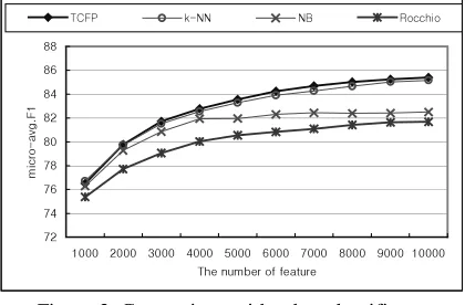
3.2.2 Comparison with other classifiers
The comparisons with other classifiers are shown in Figure 3 and Table 3. In this experiment, we used Naïve Bayes, and Rocchio classifier.
Figure 3. Comparison with other classifiers
Table 3. The top micro-average F1of each classifier
TCFP k-NN NB Rocchio
85.41 85.15 82.51 81.68
The result shows that TCFP produced the higher performance than the other classifiers.
3.2.3 Comparison of performances in an uneven data set, WebKB.
In the above experiments, the Newsgroup data set, which is an evenly divided data set, was used. If we use an uneven data set, we can face a problem. The cause of the problem is that a category of the larger size has more voting candidates than a category of the smaller size.
We simply modified the majority voting score calculated in TCFP algorithm by the following formula:
{
}
⋅
= [ ] max ( , ) / ( , ) ]
[ i j
c j
j votec numd c numd c
c vote
i
(9)
where num(d,cj) denotes the number of training
document in category cj.
The results of the modified algorithm are shown in Table 4. As we can see in this table, the modified TCFP algorithm performed similarly on the uneven data set, WebKB; the modified TCFP algorithm achieved the highest score.
Table 4. The top micro-average F1of each classifier
TCFP k-NN NB Rocchio k-NNFP
k-NN with reduction
86.6 84.83 85.22 85.98 82.78 81.34
3.2.4 Run-time observation
Table 5 shows the average running times in CPU seconds for each classifier on the Newsgroup data. Note that we included only testing phase with 4,000 documents.
Table 5. Average running time of each classifier
TCFP without context
Rocchio NB TCFP k-NNwith reduction
k-NN
0.69 0.8 1.22 1.38 37.97 142.5
Since the computations depend on the vocabulary sizes, we calculated the above numerical value by averaging running times from 1,000 to 10,000 terms. In Table 5, the running time of TCFP is similar to other faster classifiers: Rocchio and Naïve Bayes. Also it is about one hundred times faster than that of k-NN. Note that TCFP without contextual information is the fastest classifier.
4. Discussions
and n is the number of unique terms in the training collection. TCFP has the time complexity of O(m2). Even more, the time complexity of TCFP without contextual information is O(mc), where c is the number of categories. That is, the classification of TCFP requires a simple calculation in proportion to the number of unique terms in the test document. On the other hand, in k-NN, a search in the whole training space must be done for each test document.
The other strong points of TCFP are the simplicity of algorithm and high-performance. Since the algorithm of TCFP is very simple like k-NN, TCFP can be implemented quite easily and its training phase can also be a simple process. In our experiments, we achieved the better performance than k-NN. We analyze that our algorithm is more robust from irrelevant features than k-NN. When a document contains irrelevant features, the angle of the document vector is changed in k-NN. In TCFP, however, the irrelevant features contribute to only voting of the features. Hence TCFP decreases the bad effect of the irrelevant features.
Conclusions
In this paper, a new type of text categorization, TCFP, has been presented. This algorithm has been compared with k-NN and other classifiers. Since each feature in TCFP individually contributes to the classification process, TCFP is robust from irrelevant features. By the simplicity of TCFP algorithm, its implementation and training process can be done very easily. The experimental results show that, on the performance, TCFP is superior to Rocchio, Naïve Bayes, and k-NN. Moreover, it outperforms other classifiers for speeding classification such as k-NNFP and k-NN with reduction. In running time observation, TCFP is about one hundred times faster than k-NN. Therefore, we can use TCFP in the areas, which require a fast and high-performance text classifier.
References
Aha, D. W., Dennis K., and Marc K. A. (1991) Instance-Based Learning Algorithms. Machine Learning, vol. 6, pp. 37-66.
Akkus A. and Guvenir H.A. (1996) K Nearest Neighbor Classification on Feature Projections. In Proceedings of ICML’ 96, Itally, pp. 12-19.
Duda R.O., Hart P.E., and Stork D.G. (2001)Pattern Classification. John Wiley & Sons, Second Edition.
Hart, P. E. (1968) The Condensed Nearest Neighbor Rule. Institute of Electrical and Electronics Engineers Transactions on Information Theory. Vol.
14, pp. 515-516.
Ko Y. and Seo J. (2000) Automatic Text
Categorization by Unsupervised Learning. In Proceedings of the 18thInternational Conference on Computational Linguistics (COLING), pp. 453-459. Lewis D.D., Schapire R.E., Callan J.P., and Papka R. (1996) Training Algorithms for Linear Text Classifiers. In Proceedings of the 19th International Conference on Research and Development in Information Retrieval (SIGIR’96), pp.289-297. McCallum A. and Nigam K. (1998) A Comparison of
Event Models for Naïve Bayes Text Classification.
AAAI ’98 workshop on Learning for Text
Categorization. pp. 41-48.
Salton G. and McGill M.J. (1983) Introduction to Modern Information Retrieval. McGraw-Hill, Inc.
Salton G. and Buckley C. (1988) Term weighting approaches in automatic text retrieval. Information Processing and Management, 24:513-523.
Wilson D. R. and Martinez T. R. (2000) An Integrated Instance-based Learning Algorithm,
Computational Intelligence, Volume 16, Number 1,
pp. 1-28.
Wilson, D. R. and Martinez T. R. (2000) Reduction
Techniques for Exemplar-Based Learning
Algorithms. Machine Learning, vol. 38, no. 3, pp.
257-286.
Yang Y. (1994) Expert network: Effective and efficient learning from human decisions in text categorization and retrieval. In Proceedings of 17th International ACM SIGIR Conference on Research and Development in Information Retrieval (SIGIR’94), pp 13-22.
Yang Y. and Pedersen J.P. (1997) Feature selection in statistical learning of text categorization. In The Fourteenth International Conference on Machine Learning, pages 412-420.
Yang Y., Slattery S., and Ghani R. (2002) A study of approaches to hypertext categorization, Journal of Intelligent Information Systems, Volume 18, Number 2.