Learning to Identify Student Preconceptions from Text

Learning to Identify Student Preconceptions from Text

Adam Carlson

Department of Computer Science

and Engineering

Box 352350

University of Washington

Seattle, WA 98195

[email protected]

Steven L. Tanimoto

Department of Computer Science

and Engineering

Box 352350

University of Washington

Seattle, WA 98195

[email protected]

Abstract

Automatic classification of short textual an-swers by students to questions about topics in physics, computing, etc., is an attractive ap-proach to diagnostic assessment of learning. We present a language for expressing rules that can classify text based on the presence and rel-ative positions of words, lists of synonyms and other abstractions of a single word. We also describe a system, based on Mitchell’s version spaces algorithm, that learns rules in this lan-guage. These rules can be used to catego-rize student responses to short-answer ques-tions. The system is trained on written re-sponses captured by an online assessment sys-tem that poses multiple choice questions and asks the student to justify their answers with textual explanations of their reasoning. Several experiments are described that examine the ef-fects of the use of negative data and tagging students explanations with their answer to the original multiple choice question.

1

Introduction

We are building INFACT, a software system to support teachers in performing diagnostic assessment of their stu-dents’ learning. Our work is guided by the principle that assessment should be a ubiquitous and unobtrusive part of the learning process. Since many learning experiences involve writing, we focus on the analysis of free natural language text and certain other representations of student expression and behavior. We also believe that rich assess-ment, which informs teachers about the belief states of their students, is a valuable addition to tests with a single numeric grade.

Research supported in part by the National Science Foun-dation on Grant ITR/PE 0121345.

There are several parts to our system, including an on-line textual forum for class discussions, an annotation in-terface for teachers, and tools for displaying assessment data in various formats. The philosophy behind the sys-tem is described in (Tanimoto et al., 2000). The syssys-tem facilitates small-group discussions which the teacher can monitor and intervene if there is an obvious impasse. An astute teacher with enough time can follow the discus-sions closely and observe as students make conceptual transitions.

A major motivation for the work described in this pa-per is to find a way to reduce the burden on teachers who want such diagnostic information but who cannot afford the time needed to follow each discussion closely. Our system analyzes small selections of student writing, on the order of one or two sentences, and learns rules that can be used to identify common student preconceptions. Our approach to partially-automated analysis uses text markup rules consisting of patterns in a “rule language” and classifications that may be as general as “may be of interest” to “suggests preconception P17.”

In addition to learning text markup rules for identifying preconceptions in online discussions, we are also learn-ing rules for assesslearn-ing short textual answers in an online diagnostic testing environment. This system poses ques-tions to the student and uses the results to report student preconceptions to teachers and recommend resources to the student. The system asks multiple choice or numeric content questions and then, based on the response asks a short-answer follow-up question allowing the student to explain their reasoning. In this paper, we describe the re-sults of applying our rule learning system to classifying the responses to these follow-up questions.

clas-sification rules. Finally, we describe the empirical results of our experiments with this technique.

2

Related Work

There have been a number of approaches to essay and free-response grading. Burstein et al. (1999) developed a system that uses a per-question lexicon and broad-coverage parser to analyze free-response answers on a sentence-by-sentence basis. It determines whether the re-sponses contain items from a rubric describing specific points a student must touch upon in their answer. This system uses a deeper semantic analysis than does ours and makes explicit use of syntactic structure. On the other hand, it requires the semi-automated construction of a lexicon for each question. Our system only requires labeled responses as training data.

The LSA group at the University of Colorado at Boul-der has developed a system based on Latent Semantic Analysis (Landauer and Dumais, 1997). It uses a text similarity metric and a corpus of essays of known quality. The system is primarily intended to identify a student’s general level of understanding of a topic and recommend an appropriate text for the student to learn from, but has also been used for essay grading (Wolfe et al., 1998). They use the similarity metric to determine whether says have enough detail in various subtopics that the es-say is expected to cover. Because of the statistical proper-ties of the singular value decomposition underlying LSA, this system requires relatively large amounts of data to be trained, and works best on long essay questions, rather than short-answer responses.

The primary difference between these approaches and ours is that these systems are intended to determine whether or not the student has discussed particular con-cepts and, in the case of the Wolfe et al. paper, the depth of that discussion. However, neither is aimed at identify-ing the specific preconceptions held by a student.

3

Text Assessment Rule Language

The language we use to describe assessment rules con-sists of several types of constraints on the text required to match the rule. The constraints are applied on a word-by-word basis to the text being tested.

The most basic constraint is the term. A term is any string of alpha-numeric characters (typically a single word).

A term abstraction is defined as any regular ex-pression that can be applied to and match a sin-gle word (i.e. that contains no whitespace). How-ever, we primarily use term abstractions to represent lists of words that will be considered interchange-able for purposes of the pattern matching. Any term

that matches any of the words in a term tion matches the term abstraction. Term abstrac-tions are typically used to represent semantic classes that might usefully be grouped together, synonyms that students tend to use interchangeably, or words a teacher might substitute for a keyword in a question. Term abstractions are created manually.

An ordering constraint is a requirement that two terms (or term abstractions) occur in a particular or-der.

In addition, an ordering constraint can have an op-tional distance requirement. The distance require-ment limits the maximum number of intervening terms that can occur between the two required terms.

Finally any number of constraints can be combined in a conjunction. The conjunction requires all its constituent constraints to be met.

For example, the requirement that “fall” comes before a class of words used to indicate a greater speed, such as “faster”, “quicker”, etc., with at most two interceding words (e.g. “a lot”), and that the string also contains the word “gravity” would appear as follows.

fall

2 TA fast gravity where

2 is an ordering constraint requiring that its arguments occur in the specified order, with at most two words separating them and TA fast is a term abstraction covering the set of words “faster”, “quicker”, etc.

3.1 Relationship to Regular Expressions

The text assessment rule language is a subset of regu-lar expressions. Terms are translated into reguregu-lar expres-sions in a straightforward manner, with the term followed by one or more non-word separator characters. Term ab-stractions are simply an alternation of a set of terms. Or-dering constraints can be achieved by concatenation. If a distance requirement is present, then that can be rep-resented with a regular expression for matching a single, arbitrary word, repeated the appropriate number of times using the min,max convention for constrained repeti-tion. The conversion of conjunctions requires a potential exponential expansion in the size of the regular expres-sion, as each possible ordering must be represented as a separate possibility in an alternation. The rule shown above can be represented by the following regular expres-sion.

(gravity s+.*fall s+( S+ s+) 0,2 (fastquick)) (fall s+gravity s+( S+ s+) 0,1 (fastquick)) (fall s+( S+ s+) 0,1 gravity s+(fastquick)) (fall s+( S+ s+) 0,2 (fastquick) s+.*gravity)

... ...

Ø Term1 <# Term2

Term1 < Term2 Term1 ^ Term2

Most Specific Most General

U

Term1 Term2

Term Abstraction Term Abstraction

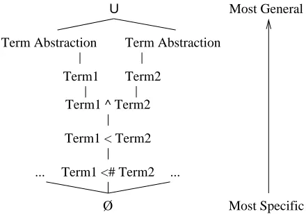
Figure 1: Generalization hierarchy for the Text Assess-ment Rule Language. Note that this represents the rules that can be obtained by successively generalizing from an example with just two terms. This is only a portion of the entire generalization lattice. For example Term1

Term3 is more general than , and more specific than Term1 alone, but unordered with respect to all the hy-potheses shown between those two.

before “falls”, after “fast” or “quick”, or as one of the words between them.

4

Learning Text Assessment Rules

The text assessment rule learner is based on Mitchell’s version spaces algorithm (Mitchell, 1982). In that frame-work, the set of all consistent hypotheses is represented and is updated as new examples are seen. In order to efficiently represent the potentially large number of con-sistent hypotheses, the hypothesis space is organized into a hierarchical lattice. The lattice is a partial ordering over hypotheses, usually defined in terms of generality. This allows the set of all consistent hypotheses to be repre-sented by storing just the boundaries, that is, the most general and most specific consistent hypotheses. Each time a new positive example is presented, any hypothesis in the specific boundary set that is inconsistent with that example is generalized to the most specific generalization that covers the new example. Conversely, a negative ex-ample causes hypotheses in the general boundary set to be minimally specialized to exclude the example. If the specific and general boundary sets ever cross, then the version space is said to collapse. In order to implement this algorithm, a generalization hierarchy must be defined over the language being learned.

4.1 Generalization Hierarchy

The version spaces algorithm requires a partial order over hypotheses. The Text Assessment Rule Language gener-alization hierarchy is shown in figure 1.

The figure shows the possible generalization steps that may be taken when an initial example consisting of two words is presented. If a subsequent example contains both words at a greater distance, the distance constraint may be relaxed. If the distance passes a fixed threshold, the distance constraint is removed completely. An exam-ple containing both words in the opposite order will cause the ordering constraint to be replaced by a conjunction. Given a conjunction, examples containing only some of the conjuncts will result in the removal of those that don’t occur. If an example doesn’t contain a term that appears in a rule, but does contain another term that is covered by the same term abstraction, the term in the rule is replaced with the term abstraction.

The initial most specific hypothesis that will match any example is the conjunction of the pairwise ordering con-straints over all pairs of words in the example. Start-ing from that initial hypothesis, the generalization pro-cess can traverse up the partial lattice shown in figure 1 for each of these pairwise ordering constraints separately. Generalization of terms to term abstractions can also oc-cur at any time. For example “A1 B C” results in the hypothesis A1

0 B A1

1 C B

0 C. If the next example is “C A2 D B” and A1 and A2 are both in term abstraction TA A, then this will result in the hypothesis

C TA A

1 B. Thus the conversion of A1 to a term abstraction, the relaxing of the distance requirement be-tween A and B and the removal of ordering constraints on C all happen simultaneously.

4.2 Disjunctions and Negative Examples

One disadvantage of lazy disjunction is that it is order dependent. If two examples can be generalized, they will be. That generalization will mean the exclusion from the resulting hypothesis, H, of terms that do not appear in both examples. A later example containing one of those terms may not be generalizable with hypothesis H even though it contains terms in common with one of the ex-amples leading to H. This order dependence can be prob-lematic. Essentially, generalization continues until an ex-ample with no terms in common with all prior exex-amples is seen, since shared terms would allow for generaliza-tion. At that point, a new disjunct is created and the process continues. This results in learning rules with disjuncts that contain one or two very common words. While we eliminate stop words in preprocessing, there re-main common content words that appear in many exam-ples but don’t relate to the concept we are trying to learn. Examples that, conceptually, form separate disjuncts are united by these red herrings. Furthermore, examples that might lead to useful generalization can be separated into different disjuncts by their coincidental similarities and dissimilarities. Our solution to this involves reducing over-generalization by using negative examples.

Typically, the version space algorithm maintains spe-cific and general boundary sets and updates the appro-priate one depending on the class of the training exam-ple. However, because the open-ended text domain is essentially infinite, and our rule language doesn’t allow directly for either disjunction or negation, the general boundary set is unrepresentable (Hirsh, 1991). Instead, we use a variant of a method proposed by Hirsh (1992) and Hirsch et al. (1997) for maintaining a list of nega-tive examples instead of a general boundary set. Nega-tive examples are stored explicitly. Members of the spe-cific boundary set that match any negative example are discarded. If no members remain in the specific bound-ary set, then the version space has collapsed. Without negative examples, we often see rules containing a single frequently occurring word. This precludes more useful generalization over disparate disjuncts. However, since common words are likely to appear in negative exam-ples as well as positive ones, such red herring rules are ruled out. Essentially, by lowering the bar before a ver-sion space would collapse, negative examples help reduce over-generalization.

In order to classify a new example, it is first tested against the specific boundary set. If all the hypotheses classify it as positive then the example is classified as positive. Otherwise, an attempt is made to add the ex-ample to the version space, on the assumption that it is positive. If that causes the version space to collapse, then the assumption is false and the example is classified as being negative. Otherwise, the version space is unable to classify the example with certainty.

5

Experiments

We use data from Diagnoser, a web-based system for diagnosing student preconceptions (Hunt and Minstrell, 1994) to test our rule learner. This assessment system has two types of questions, domain-specific base questions, which can be multiple choice or numeric, and secondary follow-up questions, which can be multiple choice or free text. The answers to the base questions are designed to correlate with common student preconceptions and the secondary questions are used to confirm the system’s di-agnosis. The system includes a database of common preconceptions that has been developed over a period of years (Hunt and Minstrell, 1996). The system primar-ily uses multiple choice follow-up questions, with just a handful of text-based ones. The developers would like to use more textual questions, but don’t currently do so due to a lack of automatic analysis tools.

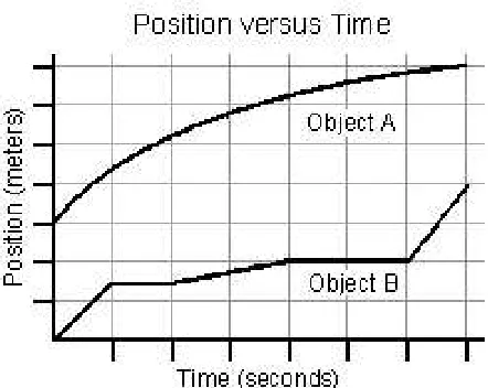
Our data consist of student answers to one of these short-answer questions. The base question is shown in figure 2. The follow-up question just asks the student to explain their reasoning. We used the students’ answers to the base question to classify the responses into three cat-egories, one for each of the three possible answers to the base question. According to the system documentation, the first answer is predictive of students who fail to dis-tinguish position and speed (Ppos-speed). Presumably, these students reported that the motion represented by the top line had a higher speed because the line is phys-ically higher. The second answer indicates that students haven’t understood the notion of average speed and are just reporting a comparison of the final speeds

(Pfinal-avg). The third answer corresponds to the correct analysis

of the question (Pcorrect). Both objects travel the same total distance in the same time, and neither ever moves backwards, so they have the same average speed.

We analyzed the text of responses to confirm that the students’ descriptions of their reasoning matched the pre-conception predicted by system based on their multiple choice answer. We found that it was necessary to cre-ate two additional classes. One class was added for students who wrote that they had guessed their answer or otherwise gave an irrelevant answer in the free text (Pmisc). Another class corresponded to a preconcep-tion that wasn’t explicitly being tested for but which was clearly indicated by some students’ responses. The ex-planations of several students who chose answer A in-dicate that they didn’t confuse position and speed. In-stead, they tried to compute the average speed of each object, but ignored the initial conditions of the system, in which object A is already 3 units ahead of object B

(Pini-tial). Thus simply relying on the multiple choice answers

Figure 2: Students were asked to explain their reasoning in answering this question

Compare the average speeds of the two objects shown in the graph above.

a) The average speed of A is greater. b) The average speed of B is greater. c) They have the same average speed.

answered B tended to be confused about the notion of average speed, few of them specifically reported consid-ering the final speeds. Rather, many of them commented that object A’s motion was smooth, while object B moved in fits and starts. The system explictly predicts a confu-sion of average speed with final speed. This shows that the vocabulary of the textual description of the precon-ception (e.g. “final speed”) isn’t necessarily a good indi-cator of the way student’s will express their beliefs.

There were 88 responses to the secondary question. Based solely on the answers to the base question, there were 61 answers classified as Ppos-speed, 15 were

Pfinal-avg and 12 were Pcorrect. After our manual

anal-ysis, the breakdown was 43 Ppos-speed answers, 10

Pfinal-avg answers, 5 Pinitial answers, 9 Pcorrect

an-swers and 21 Pmisc anan-swers.

As a baseline for comparison with the performance of our learned rules, we computed precision, recall and F-score measures for simply labeling each textual re-sponse with the preconception predicted by the student’s answer to the base question. Precision is correct posi-tives over correct posiposi-tives plus incorrect negaposi-tives (i.e. false positives). Recall is correct positives over all pos-itives (correct + incorrect.) The F-score is 2*preci-sion*recall/(precision+recall). These results are shown in table 1. Note that each row of the table shows the break-down of all 88 examples with respect to the classification of a particular preconception. Thus each row represents the performance of a single binary classifier on the entire

dataset. The recall is always 1.000 or 0.000 because of the way the data are generated. The predictions implied by the students’ answers to the base question are used and only when their explanation indicated otherwise are they reassigned to a different preconception class. Thus for those classes that were contemplated by the creator of the base question, all positive examples were correctly labeled. Conversely, for preconceptions that weren’t in-cluded in the base question formulation, no positive ex-amples are correctly identified.

Because we have very little data in some categories — as few as five examples for one class and nine for another — we use a leave-one-out training and testing regime. For each class, we construct a data set in which exam-ples from that class are labeled positive and all other ex-amples are labeled negative. We then cycle through ev-ery example, training on all but that example and testing that example. Since our goal is to identify answers that indicate a particular preconception, we’re primarily con-cerned with true and false positives. We report the num-ber of examples correctly and incorrectly labeled as well as the number of examples that the version space was un-able to classify. Precision is calculated the same way, but recall is now calculated as correct positives over the sum of correct, incorrect and unclassified positive examples.

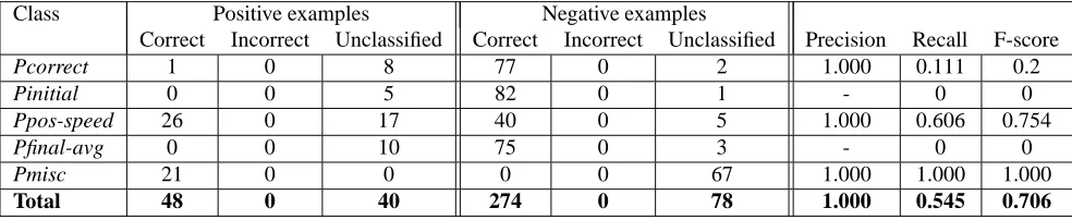
Our initial results, shown in table 2, show that the algo-rithm is able to correctly label 48 of the 88 examples and mislabeled none. While the precision of the algorithm is excellent, the recall needs improvement. The results also show that the behavior varies widely from one class to another. Clearly, for some preconceptions, the algorithm isn’t generalizing enough.

Examining the rules produced by the algorithm, we found that part of the problem is the existence of very similar answers in different classes. In particular, the

Pinitial class consists of answers where the student

Class Positive examples Negative examples

Correct Incorrect Correct Incorrect Precision Recall F-score

Pcorrect 9 0 76 3 0.750 1.000 0.857

Pinitial 0 5 83 0 - 0.000 0.000

Ppos-speed 44 0 27 17 0.721 1.000 0.838

Pfinal-avg 9 0 73 6 0.600 1.000 0.750

Pmisc 0 21 67 0 - 0.000 0.000

Total 62 26 326 26 0.705 0.705 0.705

Table 1: Results obtained by only using the students’ answer on the base question to label their short answer question. The first two columns show the number of positive examples that are correctly and incorrectly labeled, the second two columns show the number of negative examples that are correctly and incorrectly labeled.

Class Positive examples Negative examples

Correct Incorrect Unclassified Correct Incorrect Unclassified Precision Recall F-score

Pcorrect 1 0 8 77 0 2 1.000 0.111 0.2

Pinitial 0 0 5 82 0 1 - 0 0

Ppos-speed 26 0 17 40 0 5 1.000 0.606 0.754

Pfinal-avg 0 0 10 75 0 3 - 0 0

Pmisc 21 0 0 0 0 67 1.000 1.000 1.000

Total 48 0 40 274 0 78 1.000 0.545 0.706

Table 2: Results from the first leave-one-out experiment. The first three columns are the number of correctly and incorrectly classified and unclassifiable positive examples, the next three columns are the same for negative examples. The final columns show the precision, recall and F-score of the system on the positive examples only.

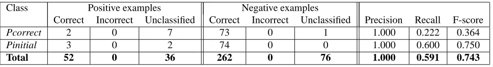
to three, which, while not much in absolute terms, repre-sents a recall of 60% with no reduction in precision. The

Pcorrect class had more limited gains, going from one

to two correctly labeled examples, again with no loss of precision.

These improvements led us to ask whether negative examples were limiting generalization in other cases as well. In order to test this, we ran the same leave-one-out experiment using only positive examples to test the recall of the rules we were producing and then used all the pos-itive examples with no negative examples to learn a set of rules and tested those rules on all the negative examples. The results of this experiment are shown in table 4. The performance of the algorithm has improved significantly. The recall on positive examples for this trial is 89% and there are still no false positives.

While these results are promising, we would like to be able to make use of negative examples in our sys-tem. In the process of analyzing student response data by hand, we found that it was often helpful to look at the stu-dent’s answer to the base question associated with a given follow-up question. It seemed likely that this information would also be useful to the rule learner. We added to each text response a pseudo-word indicating the student’s base question response and reran the algorithm using negative examples. We included Pcorrect data as negative exam-ples for Pinitial and vice versa because our hope was

that the use of the base response tags would allow the algorithm to create rules that wouldn’t conflict with neg-ative examples from another class because the examples would have different tags. The results are shown in ta-ble 5. For most classes, the addition of the tags improved the performance over untagged data. This is even true in Pinitial, where all the tags were wrong (since those data came from students whose base response indicated

Ppos-speed.) In this class, the addition of tags allowed

the same number of positive answers to be identified as the removal of negative evidence from the Pcorrect class did, implying that the tags served to avoid the trap of generalization-quashing negative evidence. However, in both these classes, the addition of tags led to some exam-ples being incorrectly classified instead of just remaining unclassified.

The only class where tag data posed a problem was the

Pmisc class. This is not surprising as this class contains

Class Positive examples Negative examples

Correct Incorrect Unclassified Correct Incorrect Unclassified Precision Recall F-score

Pcorrect 2 0 7 73 0 1 1.000 0.222 0.364

Pinitial 3 0 2 74 0 0 1.000 0.600 0.750

Total 52 0 36 262 0 76 1.000 0.591 0.743

Table 3: Retest of Pcorrect and Pinitial without conflicting negative evidence. Totals are carried over and revised from Table 2.

Class Positive examples Negative examples

Correct Incorrect Unclassified Correct Incorrect Unclassified Precision Recall F-score

Pcorrect 7 0 2 73 0 6 1.000 0.778 0.875

Pinitial 3 2 0 78 0 5 1.000 0.600 0.750

Ppos-speed 43 0 0 0 0 45 1.000 1.000 1.000

Pfinal-avg 5 0 5 63 0 15 1.000 0.500 0.667

Pmisc 21 0 0 0 0 67 1.000 1.000 1.000

Total 79 2 7 214 0 138 1.000 0.898 0.946

Table 4: The learner is trained using only positive examples. Positive examples are tested with the leave-one-out methodology. Negative examples are tested on rules learned with all positive examples.

different ways. Classes of this type are easy to spot and can easily be trained on untagged data. This was, in fact, the class that did the best when trained on untagged data. Had this been done, the total number of correctly classi-fied positive examples would have been 66, for a recall of 75%. The use of tag data also increases the performance of the system on negative examples to over 99%.

6

Remarks

Currently, the only processing of the student text done by the system is the removal of stopwords and stemming. It would be interesting to preprocess the text with part-of-speech tagging and syntactic and grammatical analysis, such as identification of passive or active voice or even full parsing. Because of the broad range of ways in which students express their ideas, the system may be severely hampered by limited exposure to syntactic variation. Tra-ditional NLP analyses might allow for the creation of rule analogues. For example, a rule that matched “subtract the initial position from the final position” might be mapped to another rule that could match “take the final position and subtract the initial position.” The application of such methods might be complicated by the fact that student writing is often highly ungrammatical and short-answer responses may well be more so.

Another way to improve the performance of automatic text analysis in assessing students is to take some care in constructing the problems presented to students to ease analysis of their answers. In the responses that were as-signed to Pfinal-avg, students described various qualita-tive comparisons between the two lines. The lines were labeled as Object A and Object B on the graph. In their

responses, students referred to them as “object A”, “line A”, “graph A” and just “A”. Since “A” is a common stop-word, this effected our ability to learn rules for this pre-conception. We removed “A” from our stopword list, which allowed for different rules to be learned, but also allowed other rules to include “A” when it was being used as an indefinite article. The use of part-of-speech tagging may improve this situation, but so would changing the question to label the graph in a way that would be less confusing to the system.

Key factors in the success or failure of experiments such as these are the variety of messages that must be mapped into a single category and degree to which us-age of various words and patterns of words is consis-tent in implicating one category rather than another. Ul-timately, the utility of techniques such as those we are studying may depend on the careful scoping of these cate-gories and means to bias student writing towards particu-lar styles or vocabuparticu-laries. These techniques offer one ap-proach to language analysis that lies between the purely syntactic and the thoroughly semantic ends of the spec-trum. We are optimistic about their practical potential in the realm of educational assessment.

Acknowledgements

Class Positive examples Negative examples

Correct Incorrect Unclassified Correct Incorrect Unclassified Precision Recall F-score

Pcorrect 6 1 2 79 0 0 1.000 0.667 0.800

Pinitial 3 2 0 83 0 0 1.000 0.600 0.750

Ppos-speed 33 0 11 43 0 1 1.000 0.750 0.857

Pfinal-avg 3 0 6 79 0 0 1.000 0.333 0.500

Pmisc 4 0 17 66 0 1 1.000 0.190 0.320

Total 49 3 36 350 0 2 1.000 0.557 0.715

Table 5: Leave-one-out trial using data tagged with the students’ responses to the corresponding base question.

References

Jacky Baltes. 1992. A symmetric version space algo-rithm for learning disjunctive string concepts. Techni-cal Report 92/468/06, University of Calgary, March.

Jill C. Burstein, Susanne Wolff, and Chi Lu. 1999. Using lexical semantic techniques to classify free-responses. In Nancy Ide and Jean Veronis, editors, The Depth

and Breadth of Semantic Lexicons. Kluwer Academic

Press.

Haym Hirsh, Nina Mishra, and Leonard Pitt. 1997. Ver-sion spaces without boundary sets. In Proceedings of

the Fourteenth National Conference on Artificial Intel-ligence, pages 491–496. Menlo Park, CA: AAAI Press,

July.

Haym Hirsh. 1991. Theoretical underpinnings of version spaces. In Proceedings of the Twelfth International

Joint Conference on Artificial Intelligence, pages 665–

670. San Francisco, CA: Morgan Kaufmann, July.

Haym Hirsh. 1992. Polynomial-time learning with ver-sion spaces. In William Swartout, editor, Proceedings

of the 10th National Conference on Artificial Intelli-gence, pages 117–122, San Jose, CA, July. MIT Press.

Earl Hunt and Jim Minstrell. 1994. A cognitive approach to the teaching of physics. In Kate McGilly, editor,

Classroom lessons: Integrating cognitive theory and the classroom. M.I.T. Press.

Earl Hunt and Jim Minstrell. 1996. Effective instruction in science and mathematics: Psychological principles and social constraints. Issues in education:

contribu-tions from educational psychology, 2(2):123–162.

Thomas K. Landauer and Susan T. Dumais. 1997. A so-lution to plato’s problem: The latent semantic analysis theory of the acquisition, induction, and representation of knowledge. Psychological Review, 104:211–240.

T. Mitchell. 1982. Generalization as search. Artificial

Intelligence, 18:203–226.

Steven L. Tanimoto, Adam Carlson, Earl Hunt, David Madigan, and Jim Minstrell. 2000. Computer sup-port for unobtrusive assessment of conceptual knowl-edge as evidenced by newsgroup postings. In Proc.

ED-MEDIA 2000, June.