Enhance Top down method with Meta Classification for Very Large scale Hierarchical Classification

Enhance Top-down method with Meta-Classification

for Very Large-scale Hierarchical Classification

Xiao-Lin Wang1,2_{, Hai Zhao}1,2_{, Bao-Liang Lu}1,2†

1_{Center for Brain-Like Computing and Machine Intelligence}

Department of Computer Science and Engineering, Shanghai Jiao Tong University

2_{MOE-Microsoft Key Laboratory for Intelligent Computing and Intelligent Systems}

Shanghai Jiao Tong University

800 Dong Chuan Rd., Shanghai 200240, China

[email protected],{zhaohai; blu_}@cs.sjtu.edu.cn

Abstract

Recent large-scale hierarchical classifica-tion tasks typically have tens of thousand-s of clathousand-sthousand-sethousand-s athousand-s well athousand-s a large number of samples, for which the dominant solution is the top-down method due to computa-tional complexity. However, the top-down method suffers from accuracy deficiency, that is, its accuracy is generally lower than that of the flat approach of 1-vs-Rest. In this paper, we employ meta-classification technique to enhance the classifying pro-cedure of the top-down method. We an-alyze the proposed method on the aspect of accuracy, and then test it with two real-world large-scale data sets. Our method both maintains the efficiency of the con-ventional top-down method and provides competitive classification accuracies.

1 Introduction

Test categorization, as a key technology of data mining, has received intensive study for decades. Recently, real-world applications have raised some large-scale tasks that typically have tens of t-housands of classes, where many established tech-niques such as the 1-vs-Rest multiclass classifica-tion fail due to computaclassifica-tional complexity. Mean-while, those large-scale tasks usually employ hi-erarchies to organize the huge number of class-es that they have, which providclass-es a clue to solve them. Such kind of tasks include categorizing

∗ _{This work was partially supported by the National}

Natural Science Foundation of China (Grant No. 60903119, Grant No. 61170114 and Grant No. 90820018), the National Basic Research Program of China (Grant No. 2009CB320901), the Science and Technology Commis-sion of Shanghai Municipality (Grant No. 09511502400), and the European Union Seventh Framework Programme (Grant No. 247619).

† _{Corresponding author}

patent documents into the taxonomy of Interna-tional Patent Classification (IPC) (Fall et al., 2003; Fujii et al., 2007) and categorizing web pages into the directories of Open Directory Project (ODP) or Yahoo! (Labrou and Finin, 1999; Liu et al., 2005). The existing approaches to hierarchical classifi-cation mainly fall into two categories. One cate-gory aims at raising classification accuracy, which generally takes hierarchies as additional clue for classifying a sample besides its content. Such re-searches include hierarchical support vector ma-chines (SVM) (Cai and Hofmann, 2004; Tsochan-taridis et al., 2005), hierarchical Rocchio-like clas-sifiers (Labrou and Finin, 1999), min-max mod-ular network (Lu and Ito, 2002; Lu and Wang, 2009) and ensemble classifications (Punera and Ghosh, 2008).

The other category aims at reducing computa-tional complexity. The main approach in this cat-egory is an ensemble classification method called top-down method (Bennett and Nguyen, 2009; Ce-ci and Malerba, 2007a; Koller and Sahami, 1997; Liu et al., 2005; Montejo-R´aez and Ure˜na-L´opez, 2006; Sun and Lim, 2001; Xue et al., 2008; Yang et al., 2003). Top-down method builds a tree of classifiers which is isomorphic with the hierarchy of classes.

Top-down method classifies a test sample as fol-lows. The sample is filtered down the tree of clas-sifiers from the root node. For each parent node that the sample reaches, those child nodes whose confidence values predicted by the base-classifiers exceed a predefined threshold are invoked to carry the sample on. When the sample reaches the bot-tom leaf nodes eventually, the predictions can be made (Liu et al., 2005; Montejo-R´aez and Ure˜na-L´opez, 2006; Yang et al., 2003). As this classify-ing process employs the threshold strategy of com-paring the scores with thresholds, which is named score-cut (S-cut) in the context of flat multiclass classification (Yang, 2001), we call this kind of

conventional top-down method the S-CUT Top-Down method (ScutTD) so as to distinguish it from the later variant top-down methods in this pa-per.

ScutTD is far more efficient than the normal flat approach of 1-vs-Rest in handling the classi-fication tasks that has a large number of classes. The computational complexity of 1-vs-Rest is lin-ear to the number of classes, while that of ScutTD is approximately logarithmic (Ceci and Maler-ba, 2007a; Liu et al., 2005; Wang and Lu, 2010; Yang et al., 2003). As an practical example, in an classification experiment on 492 617 training doc-uments, 275 364 test documents and 132 199 cate-gories of Yahoo!, ScutTD costs only 2.1 hours on training and 0.12 hours on classifying, while 1-vs-Rest costs 310 hours on training and 54 hours on classifying (Liu et al., 2005).

However, ScutTD has a well-known deficien-cy of classification accuradeficien-cy, that is, its perfor-mance is generally worse than the flat 1-vs-Rest approach (Bennett and Nguyen, 2009; Ceci and Malerba, 2007a; Wang and Lu, 2010; Xue et al., 2008). As a persuasive evidence, in the 2009 PAS-CAL challenge on large-scale hierarchical text 1_,

flat methods rank highest, hybrid methods rank next and top-down methods rank lowest.

The main reason for the accuracy deficiency of ScutTD is that its classifying procedure actually consists of cascaded decisions about which child nodes should be invoked from a parent node. Each of these decisions is made upon the score of lo-cal base-classifiers only, and not changeable after that. Thus a wrong decision inevitably leads to a group of wrong predictions. This problem is usu-ally called error propagation (Wang and Lu, 2010; Xue et al., 2008). Sun et al. study a special case of this problem, the wrong decision of rejecting a child node at high layers, and call it the blocking problem (Sun et al., 2004). Liu et al. compare this classifying procedure to a Pachinko-machine (Liu et al., 2005). As a solution, Ceci and Malerba has proposed a bottom-up thresholding strategy (Ceci and Malerba, 2007a)

In this paper, we propose a ‘global’ classify-ing method for top-down method to reduce its er-ror propagation. The idea is to treat combining the predictions of the base-classifiers as a meta-classification task, for which we name our method Meta-classification Top-down method (MetaTD).

1_{http://lshtc.iit.demokritos.gr/}

There is one point that needs to be clarified. There are two kinds of hierarchical classification tasks in real-world applications. One kind is mandatory leaf-node classification where only the leaf nodes are the validate labels or classes (Du-mais and Chen, 2000; Freitas and de Carvalho, 2007; Silla and Freitas, 2010). In contrast, the oth-er is non-mandatory leaf-node classification corre-spondingly, where both the internal nodes and the leaf nodes are validate labels (Lewis et al., 2004; Liu et al., 2005). In this paper, we handle the first kind of hierarchical classification – mandato-ry leaf-node classification.

The rest of paper is organized as follows. The proposed MetaTD as well as the conventional S-cutTD is formally presented in Sec. 2. We then provide some ideas on the classification accuracy of MetaTD in Sec. 3. After that we test MetaTD with two real-world data sets in Sec. 4. Finally we conclude this paper in Sec. 5.

2 Methods

In this section, we present the formal descriptions of the proposed MetaTD. We first review the con-ventional ScutTD. We then present MetaTD in de-tail. After that an example is given to illustrate MetaTD.

2.1 S-cut Top-down Method

SupposeHis a hierarchy of classes which records all the relations of parent nodes and their children,

H={(p, c)|pis a parent node, cis one of its children_} where(p, c)is called a parent-child relation. Sup-poseT,DandEare the training, development and test sets respectively.

Applying ScutTD consists of the following three steps.

First, train base-classifiers. One classifier will be trained for each parent-child relation (p, c) of the hierarchyH, noted asfc, through the

follow-ing local trainfollow-ing set,

Tpc ={(x, y)|x∈Tp,y= +1ifx∈Tc,

y=₋1otherwise} (1)

whereT_∗ is the subset of training samples that be-long to the node∗.

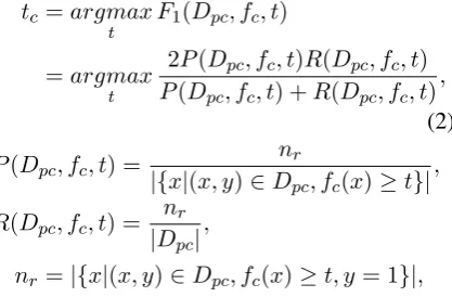
Second, find optimal thresholds for the base-classifiers. The approaches to this step actually have alternatives. Micro-F1 is taken as the

pre-cision and recall, as follows (Bennett and Nguyen, 2009; Liu et al., 2005).

tc=argmax

t F1(Dpc, fc, t)

=argmax

t

2P(Dpc, fc, t)R(Dpc, fc, t)

P(Dpc, fc, t) +R(Dpc, fc, t)

,

(2)

P(Dpc, fc, t) =

nr

|{x_|(x, y)_∈Dpc, fc(x)≥t}|

,

R(Dpc, fc, t) =

nr

|Dpc|

,

nr=|{x|(x, y)∈Dpc, fc(x)≥t, y= 1}|,

wheretcandfc are the local threshold and

base-classifier, Dpc is the local development subset

which is similar with the Tpc defined by Eq. 1),

P andRare the precision and recall, andnris the

number of correct predict labels.

Third, classify the test instances. The algorithm of this step is presented in Fig. 1. With the trained base-classifiersfcand the thresholdstc, the test set

Ecan be classified.

2.2 Meta-classification Top-down method

To describe the proposed MetaTD, we first intro-duce the definition of meta-samples as follows,

M(u, l, f_∗) = (_Mx(ux, l, f∗),My(uy, l, f∗)) (3) Mx(ux, l, f∗) ={(ni, fni(ux))|ni ∈pl}

My(uy, l, f∗) =

{

+1, l_∈uy

−1, l_̸∈uy

where M is the meta-mapping that consists of meta-inputMx and meta-output My, H is a

hi-erarchy, u = (ux, uy) is a base-sample where

ux is the input part and uy is the label set, l is

a leaf node (or a label), that is, a validate label for base-samples, pl = (n0, n1, . . . , nk)is a path

from the root to l where n0 = root, nk = l,

(ni, ni+1)∈H, andf∗are base-classifiers. However, the above definition yields one meta-sample for each class, which may cause a problem of computational complexity on large-scale tasks. Hence a method of selecting label candidates for each base-sample is employed so that only a small fraction of labels need to be delivered into meta-classification. We note this selection method as L(ux, f∗, H).

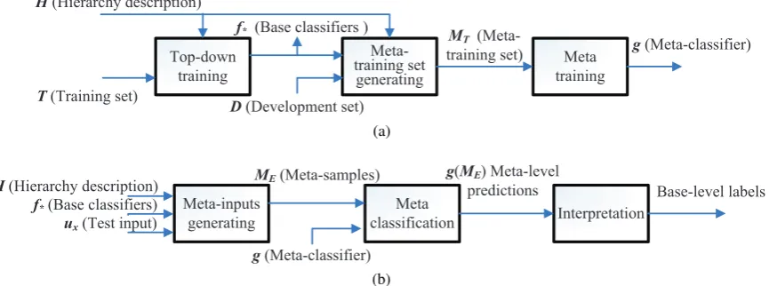
MetaTD is based on the above two settings, and its workflow is described in Fig. 2.

Require: a test instancex

a hierarchyH={(p, c)|(p, c)is a parent-child} base-classifiers{fc|(p, c)∈H}

thresholds{tc|(p, c)∈H}

Ensure: a predicted label sety q ←[Root],y← {}

whileqis not emptydo

p_←pop out the first item ofq

ifpis a leaf nodethen y_←y_{∪ {}p_}

else

for allc,(p, c)∈Hdo sc←fc(x)

ifsc≥tcthen

appendcintop

end if end for end if end while return y

Figure 1: ScutTD algorithm

The training phase consists of three steps as fol-lows,

1. Train base-classifiersf_∗on a training data set T, which is the same with ScutTD.

2. Construct a meta-training set with the base-classifiers and a development setD,

MT =∪u∈D{M(u, l, f∗, H)|l∈L(ux, f∗, H)}.

3. Train a meta-classifiergonMT.

The whole training phase requires the base-level training setT and development setD, the descrip-tion of the hierarchy H, and produces a set of base-classifiersf_∗and a meta-classifierg.

The classifying phase also consists of three steps as follows,

1. Construct a group of meta-samples from a test base-sampleux(its labeluyis unknown),

ME ={Mx(ux, l, f∗)|l∈L(ux, f∗, H)}.

2. Present these samples to the meta-classifierg,

g(ME) ={g(Mx(ux, l, f∗))|l∈L(ux, f∗, H)} =_{gux,l|l∈L(ux, f∗, H)}.

Top-down training

Meta-training set

generating

Meta training

T(Training set)

H(Hierarchy description)

f* (Base classifiers )

D(Development set)

MT

(Meta-training set) g(Meta-classifier)

(a)

Meta-inputs generating

Meta classification

f* (Base classifiers)

ME(Meta-samples) g(ME) Meta-level predictions

Interpretation

Base-level labels

ux(Test input)

H(Hierarchy description)

g(Meta-classifier) (b)

Figure 2: Workflows of meta-classification top-down method: (a) training phase; (b) classifying phase.

straightforward, and just outputs the labels with large scores. The practical interpreta-tion depends on the data sets, and will be de-scribed in the section of experiments.

The remained problems now are how to imple-ment meta-sample representations Mx(ux, l, f∗) and selection of label candidates L(ux, f∗, H), which are solved in the next two subsections.

2.2.1 Representations of Meta-samples

In this subsection, the meta-samples will be made into real numerical vectors that are ready to be used by meta-classifiers. We use sparse vector to represent meta-samples through the following steps:

First, encode the scores of the related base-classifiers into a sparse vector. All the nodes ex-cept the root are numbered with integers, which serve as the dimensions of the sparse vector.

Second, augment the representations with the features about the global attributes of the root-to-leaf paths in the hierarchy. The purpose of this step is to raise classification accuracy, as these global attributes may be helpful to decide whether a path is true. The following three additional features are used according to our pilot experiments,

1. theaveragescore of nodes along a path; 2. theminimumscore of nodes along a path; 3. the fraction of nodes whose scores exceed the

thresholds employed in ScutTD, named pass-rate.

In the end, the values of meta features are trans-ferred into a sensible interval in order to fit the training of meta-classifiers (Liu, 2005; Liu et al.,

2004). Two types of transformation functions are used according to our pilot experiments. For the additional features, the following standard scaling function is used,

zs=

s₋µs

σs

where sis the value of an additional feature, µs

andσsare the corresponding mean and variance.

For the basic features, the following sigmoid function is used,

zs=

1 1 +e−(s−µs)

wheresis a score at a noden, and µs is the

av-erage score at noden. This function is a simpli-fication of the Platt’ sigmoid fitting (Platt, 1999; Cesa-Bianchi et al., 2006), and it is more robust than the original one in the context of hierarchical classification according to our pilot experiements.

2.2.2 Selection of Label Candidates

How should label candidates be selected? In fact, the method of selecting label candidates is kind of like a classification method as both of them take in samples and give out the labels most likely to be right. However, the method of selecting la-bel candidates should output more lala-bels than a normal classifying method, in order to provide a wider coverage on truly correct ones. To find such a ‘loose’ classifying method, we refer to flat multi-class multi-classification where another threshold strat-egy of Rank-cut (R-cut), besides the S-cut intro-duced above, is also widely used (Montejo-R´aez and Ure˜na-L´opez, 2006; Yang, 2001). R-cut is to accept the topr labels with the highest confident scores, whereris a predefined integer.

5RRW

Q Q

Q Q Q Q

Q

(a)

5RRW

V V

V V V V

V

IDOVH

IDOVH

WUXH WUXH

(b)

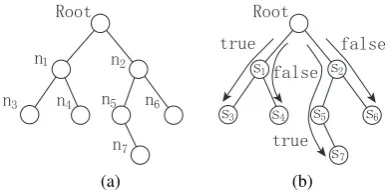
Figure 3: An illustration of solving hierarchical classification with MetaTD: (a) the class hierar-chy; (b) the paths as meta-samples.

invoked from their parent node regardless of their scores, and the rest procedure is the same with S-cutTD (see Fig. 1). We name this method RS-cutTD, and employ it to select label candidates in the pro-posed MetaTD. Note that RcutTD has been dis-cussed before and is considered improper for the classifying procedure of the top-down method (Li-u et al., 2005).

2.3 Illustration of Meta-classification Top-down Method

In this subsection we illustrate MetaTD with an example. Suppose a hierarchical classification task has the hierarchy of classes shown by Fig. 3a, wheren0is the root, and the leaf nodesn3,n4,n6

andn7are validate labels.

Further suppose that a tree of base-classifiers have been built through the top-down training. Here comes a sample with n3 and n7 as its

cor-rect labels. Fig. 3b shows that each base-classifier yields a relevant scoresi.

MetaTD converts each possible label (or leaf n-ode) into a meta-sample – the target is whether this leaf node is a correct label and the features are the scores of the base-classifiers along the path (Fig. 3b). For this example, the following four meta-samples can be generated,

true n0 → (n1, s1) →(n3, s3)

false n0 → (n1, s1) →(n4, s4)

true n0 → (n2, s2) →(n5, s5) →(n7, s7)

false n0 → (n2, s2) →(n6, s6).

(4) These meta-samples are then interpreted into numerical sparse vectors. Suppose that n1 ton7

are numbered with integers1–7, then the numeri-cal sparse vectors can be generated (see Tab. 1).

With more samples like above, a meta-classifier can be trained. Later this meta-meta-classifier

No. Basic Extension

1 1:s1a 3:s3 8:a13b 9:m13 10:p13

2 1:s1 4:s4 8:a14 9:m14 10:p14

3 2:s2 5:s5 7:s7 8:a257 9:m257 10:p257

4 2:s2 6:s6 8:a26 9:m26 10:p26

a_{dimension:value} b_a

i1i2...ik,mi1i2...ik,pi1i2...ikdenote the average, minimum, and pass-rate ofsi1,si2 . . .sik respec-tively.

Table 1: Representing meta-samples with sparse vectors

can be applied to the meta-samples made from a base-level test sample to pick out the right labels. In this way, MetaTD fulfills the original base-level classifying task.

3 Accuracy Analysis

The classification accuracy of top-down method-s imethod-s actually not very clear or predictable. To our best knowledge, no strict accuracy analyses on the conventional ScutTD have been reported yet. Here we just provide some general ideas about the com-parison of accuracy between MetaTD and ScutTD. First, whether pruning possible labels with R-cutTD or not has minor impact on the overall clas-sification result. The labels rejected by RcutTD all have quite low scores on some parent-child re-lations and are very likely to be filtered out by the successive meta-classifier.

Second, ignoring the impact of selecting label candidates, the conventional top-down method of ScutTD can be actually seen as a weak meta-classifier in the framework of MetaTD. Suppose here is a meta-sample (a sparse vector),

(n1:z1, n2:z2, . . . , nk:pk, na:za, nm:zm, np:zp)

whereniandpi are a node number and its value,

and na,nm,np are the additional features. Then

ScutTD works like, Output=

{

True ifpi> ti for alli= 1 . . . k

False otherwise

whereti is the threshold of nodeni. Clearly this

formula is a cascaded of binary decisions, which is weaker than some common classifiers such as weighted voting.

4 Experiments

Data No. Sample Feature Class Train. Dev. Test No. Avg.a_{No. Avg.}b

LSHTC 93k 34k 34k 381k 173 12k 1.0 NTCIR 2 762k 374k 359k 694k 108 49k 2.7

a_{average features per sample, that is, average}

u-nique terms per document.

b_{average labels per sample.}

Table 2: Statistical information of data sets

report the comparison with flat 1-vs-Rest approach on several subsets.

4.1 Experimental Settings 4.1.1 Data Sets

Two real-world data sets, the data set of web pages in the PASCAL2 Large-scale Hierarchical Tex-t ClassificaTex-tion challenge (LSHTC)2 _{and the data}

set of patent documents from NII Test Collection for IR Systems Project (NTCIR)3_{, are used in our}

experiments.

The PASCAL2 Large-scale Hierarchical Text Classification (LSHTC) challenge is held at 2009, aimed at promoting the study of classification methods for large hierarchies. The challenge at-tracts 19 participants with a variety of approach-es (Kosmopoulos et al., 2010).

International Patent Classification (IPC) is a real-world taxonomy maintained by World Intel-lectual Property Organization (WIPO)4_{. The data}

set that we use is provided by NTCIR which is freely available for research purpose (Fall et al., 2003; Fujii et al., 2007). This data set consists of 3 496 137 Japanese patent documents submitted to Japan Patent Office from 1993 to 2002.

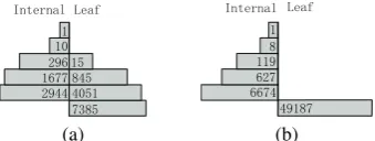
The statistics of two data sets and their hierar-chies are presented in Tab. 2 and Fig. 4. Note that LSHTC’s is a single-labeled task while NTCIR’s is a multi-labeled ones.

4.1.2 Performance Measurement and Baseline Methods

Different performance measurements and baseline methods are adopted for the two data sets due to their difference of single-label and multi-label. NTCIR is multi-labeled, so the most commonly used criterion for general multi-labeled classifica-tions, micro-F1, is taken as the performance

mea-surement. ScutTD is taken as the baseline method.

2_{http://lshtc.iit.demokritos.gr/} 3_{http://research.nii.ac.jp/ntcir/} index-en.html

4_{http://www.wipo.int/classifications/} ipc/en/

74 69 53

21

10

82 77 62 25 ,QWHUQDO /HDI

(a)

82 60

44 19

10

100

,QWHUQDO /HDI

(b)

Figure 4: Number of internal and leaf nodes at each level of the hierarchy: (a) LSHTC; (b) NT-CIR.

LSHTC is single-labeled, so accuracy is taken as the performance measurement. However, there is a problem about baseline method as ScutTD is not proper for single-labeled task. As a matter of fact, single-labeled hierarchical classifications are easier than multi-labeled ones, and it is natural to activate the child node with the largest score dur-ing top-down classification, like (Koller and Sa-hami, 1997). This method happens to be RcutTD with the parameterr=1. In addition to this base-line method, the evaluation records of LSHTC are also used for comparison.

4.1.3 Settings of MetaTD

The representation of meta-samples follows the description in Sec. 2.2.1. RcutTD is employed to select label candidates as described in Sec. 2.2.2. We set the parameter r=2 due to a trade-off be-tween classification accuracy and time cost ac-cording to several pilot experiments.

The recent implement of SVM, Liblinear, is adopted as the meta-classifier (Fan et al., 2008).

Meta-to-base interpreters are needed to transfer the meta-level predictions into base-level labels. LSHTC is single-labeled, so it’s natural to take the label with the largest meta-level scores. NTCIR is multi-labeled, and the strategy of S-cut in flat multi-class classification is employed.

4.1.4 Other Settings

The bag-of-word model with the term weight of TFIDF is adopted as the base-level sample repre-sentation in this paper (Sebastiani, 2002). To han-dle the Japanese text in the NTCIR’s data set, we use the segment tool of Chasen5_{(Jin et al., 2010),}

and remove the function words from the result. The base-level classifier is SVMlight_{with linear}

kernel. The default cost factor of SVMlight_{is used}

on NTCIR, while the cost factors are tuned by the development sets on LSHTC.

LSHTC, 12 294 classes

Rank Method Acc. Group

1 Not reported 0.4676 alpaca 2 Committees of flat approaches 0.4632 jhuang

MetaTD 0.4513

3 Flattened Top-down method 0.4433 arthur. 4 Centroid-based classifier 0.4431 XipengQiu 5 Deep Classification 0.4317 Turing 6 Not reported 0.4270 Dyakonov

RcutTD 0.4262

7 Flattened Top-down method 0.4152 logicators

11 k-NN 0.4023 NakaCristo

Table 3: Classification accuracies on single-labeled LSHTC as well as its challenge records

NTCIR, 49 187 classes Method Micro-F1

ScutTD 0.272

MetaTD 0.426

Table 4: Classification accuracies on the multi-labeled data set of NTCIR

The experiments are run on four 64-bit comput-ers with multi-core 1.9GHzAMD CPUs. All the experiments require actually up to 8Gmemory ac-cording to our observation.

4.2 Performance on Entire Data Sets

In this subsection we compare MetaTD with base-line methods on the entire data sets of LSHTC and NTCIR from the aspects of accuracy and efficien-cy.

4.2.1 Accuracy Comparisons

The experimental results on the single-labeled L-SHTC as well as the challenge records are pre-sented in Tab. 3. MetaTD turns out to be be-tween the second and third place, while the base-line method of RcutTD ranks between the sixth and seventh place. The method at the second place is a committee of two flat approaches – variants of the OOZ algorithm (Madani and Huang, 2008) and the passive-aggressive algorithm (Crammer et al., 2006). The methods at both the third and sev-enth places are both top-down methods enhanced by flattening the original hierarchy. Deep classifi-cation ranks at the fifth place (Xue et al., 2008). In short, MetaTD outperforms the conventional and several variant top-down methods.

The results on the multi-labeled NTCIR are pre-sented in Tab. 4. MetaTD achieves a much higher micro-F1than the baseline method of ScutTD.

Method Training Classify.a

LSHTC, 12 294 classes

RcutTD Train base-classifiers 10h 0.108 MetaTD Train base-classifiers 17h 0.131

Prepare meta-train. set 1h

Meta-training 18s

NTCIR, 49 187 classes Scut/MetaTD Train base-classifiers 261h

ScutTD Find optimal thresholds 4h 0.029 Meta-learning Prepare training set 12h 0.062

Meta-training 466s

a_{seconds per sample}

Table 5: Time costs of training and classifying with conventional top-down methods and MetaT-D.

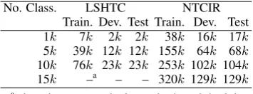
No. Class. LSHTC NTCIR

Train. Dev. Test Train. Dev. Test 1k 7k 2k 2k 38k 16k 17k

5k 39k 12k 12k 155k 64k 68k

10k 76k 23k 23k 253k 102k 104k

15k –a – – 320k 129k 129k

a_{there is not enough classes in the original data}

set.

Table 6: Numbers of classes and samples at the subsets of LSHTC and NTCIR

4.2.2 Efficiency Comparisons

The training and classifying time costs of MetaTD and baseline methods are presented in Tab. 5. In the training phrase, training base-classifiers caus-es most time cost. The additional cost of meta-classification MetaTD is only 5%–10% of that cost. Meta-training unexpectedly costs very lit-tle time, while preparing meta-training sets costs most additional time cost.

On the aspect of classifying, the time cost of MetaTD is about twice as much as the convention-al top-down methods. According to our observa-tion, considerable time is spent on reading samples and loading classifiers.

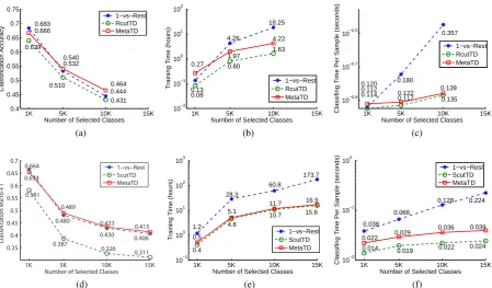
4.3 Comparison with Flat Approach of 1-vs-Rest on Subsets

In this subsection we compare the performance of top-down methods with the flat approach of 1-vs-Rest multiclass classification. Given the great computational complexity of the flat approach, several subsets are made from the entire data sets of LSHTC and NTCIR through randomly picking up classes and samples (see Tab. 6).

1K 5K 10K 15K 0.4 0.45 0.5 0.55 0.6 0.65 0.7 0.75

Number of Selected Classes

Classification Accuracy 0.683 0.639 0.666 0.532 0.510 0.540 0.444 0.431 0.464 1−vs−Rest RcutTD MetaTD (a)

1K 5K 10K 15K

10−2 10−1 100 101 102

Number of Selected Classes Training Time (hours) _0.13

0.08 0.27 4.26 0.80 1.97 18.25 1.63 4.22 1−vs−Rest RcutTD MetaTD (b)

1K 5K 10K 15K

10−0.9 10−0.7 10−0.5

Number of Selected Classes

Classifing Time Per Sample (seconds)

0.114 0.112 0.120 0.180 0.117 0.122 0.357 0.135 0.139 1−vs−Rest RcutTD MetaTD (c)

1K 5K 10K 15K

0.35 0.4 0.45 0.5 0.55 0.6 0.65 0.7

Number of Selected Classes

C lassificati on Micr o-F1 0.664 0.581 0.654 0.480 0.387 0.489 0.430 0.326 0.433 0.406 0.311 0.413 1−vs−Rest ScutTD MetaTD (d)

1K 5K 10K 15K

10−1 100 101 102 103

Number of Selected Classes

Training Time (hours)

1.2 0.4 0.5 28.3 4.6 5.1 60.8 10.7 11.7 173.7 15.6 16.9 1−vs−Rest ScutTD MetaTD (e)

1K 5K 10K 15K

10−2 10−1 100

Number of Selected Classes

Classifing Time Per Sample (seconds)

0.038 0.014 0.022 0.066 0.019 0.029 0.128 0.022 0.036 0.224 0.024 0.039 1−vs−Rest ScutTD MetaTD (f)

Figure 5: Performance comparison of flat 1-vs-Rest approach, conventional top-down methods and MetaTD on subsets of various sizes: (a) through (c) for LSHTC; (d) through (f) for NTCIR.

taken as the base-classifier.

The experiment results are presented in Fig. 5. On the aspect of classification accuracy, MetaTD catches up with the 1-vs-Rest approach. In partic-ular, MetaTD slightly outperforms 1-vs-Rest ap-proach on both data sets when the number of class-es exceeds 5 thousands.

On the aspect of computational complexity, MetaTD is close to the conventional top-down methods, and they all show a great superiority over the 1-vs-Rest approach on both training and clas-sifying as expected.

5 Conclusions

In this paper, we propose a meta-learning top-down method (MetaTD) in order to reduce the er-ror propagation of the conventional ScutTD while remain its capability for large-scale hierarchical classification. In the experiments, MetaTD outper-forms ScutTD and catches up with the flat 1-vs-Rest approach on classification accuracy. On the aspect of computational complexity, MetaTD only costs 5%-10% extra time in training and classify-ing, so it is suitable for most applications where ScutTD are being used.

References

P.N. Bennett and N. Nguyen. 2009. Refined expert-s: improving classification in large taxonomies. In

Proc. of SIGIR’09, pages 11–18. ACM.

L. Cai and T. Hofmann. 2004. Hierarchical docu-ment categorization with support vector machines. InProc. of ACM international conference on infor-mation and knowledge management, pages 78–87. ACM.

M. Ceci and D. Malerba. 2007a. Classifying web doc-uments in a hierarchy of categories: a comprehen-sive study. Journal of Intelligent Information Sys-tems, 28(1):37–78.

M. Ceci and D. Malerba. 2007b. Classifying web doc-uments in a hierarchy of categories: a comprehen-sive study. Journal of Intelligent Information Sys-tems, 28(1):37–78.

N. Cesa-Bianchi, C. Gentile, and L. Zaniboni. 2006. Hierarchical classification: combining Bayes with SVM. InProc. of ICML’06, pages 177–184. ACM.

K. Crammer, O. Dekel, J. Keshet, S. Shalev-Shwartz, and Y. Singer. 2006. Online passive-aggressive al-gorithms. Journal of Machine Learning Research, 7:551–585.

C.J. Fall, A. T¨orcsv´ari, K. Benzineb, and G. Karetka. 2003. Automated categorization in the internation-al patent classification. InACM SIGIR Forum, vol-ume 37, pages 10–25. ACM.

R.E. Fan, K.W. Chang, C.J. Hsieh, X.R. Wang, and C.J. Lin. 2008. LIBLINEAR: A library for large linear classification. Journal of Machine Learning Research, 9:1871–1874.

AA Freitas and A.C. de Carvalho, 2007. A Tutorial on Hierarchical Classification with Applications in Bioinformatics., pages 175–208. IGI Publishing.

A. Fujii, M. Iwayama, and N. Kando. 2007. Introduc-tion to the special issue on patent processing. In-formation Processing & Management, 43(5):1149– 1153.

Gang Jin, Qi Kong, Jian Zhang, Xiaolin Wang, Con-g Hui, Hai Zhao, and Bao-LianCon-g Lu. 2010. Multi-ple strategies for NTCIR-08 patent mining at BCMI. In Proc. of the 8th NTCIR workshop meeting on e-valuation of information access technologies, pages 303–308.

D. Koller and M. Sahami. 1997. Hierarchically classi-fying documents using very few words. InProc. of ICML’97, pages 170–178.

A. Kosmopoulos, E. Gaussier, G. Paliouras, and S. Aseervatham. 2010. The ECIR 2010 large scale hierarchical classification workshop. InACM SIGIR Forum, volume 44, pages 23–32. ACM.

Y. Labrou and T. Finin. 1999. Yahoo! as an ontology: using Yahoo! categories to describe documents. In

Proc. of the eighth international conference on In-formation and knowledge management, pages 180– 187. ACM.

D. D. Lewis, Y. Yang, T. G. Rose, and F. Li. 2004. Rcv1: A new benchmark collection for text catego-rization research. Journal of Machine Learning Re-search, 5:361–397.

C. L. Liu, H. Hao, and H. Sako. 2004. Confidence transformation for combining classifiers. Pattern Analysis & Applications, 7(1):2–17.

T. Y. Liu, Y. Yang, H. Wan, H. J. Zeng, Z. Chen, and W.Y. Ma. 2005. Support vector machines clas-sification with a very large-scale taxonomy. ACM SIGKDD Explorations, 7(1):36–43.

C. L. Liu. 2005. Classifier combination based on confidence transformation. Pattern Recognition, 38(1):11–28.

B.L. Lu and M. Ito. 2002. Task decomposition and module combination based on class relations: A modular neural network for pattern classification.

IEEE Tran. on Neural Networks,, 10(5):1244–1256.

B.L. Lu and X.L. Wang. 2009. A Parallel and Modular Pattern Classification Framework for Large-Scale Problems. Chen C. H. editor, Handbook of Pat-tern Recognition and Computer Vision (4th Edition), pages 725–746.

O. Madani and J. Huang. 2008. On updates that con-strain the features’ connections during learning. In

Proceeding of SIGKDD’08, pages 515–523. ACM.

A. Montejo-R´aez and L. Ure˜na-L´opez. 2006. Se-lection strategies for multi-label text categorization.

Advances in Natural Language Processing, pages 585–592.

J. Platt. 1999. Probabilistic outputs for support vec-tor machines. Bartlett P., Schoelkopf B., Schurmans D., Smola, A. J. editor, Advances in Large Margin Classifiers, pages 61–74.

K. Punera and J. Ghosh. 2008. Enhanced hierarchical classification via isotonic smoothing. InProceeding of the 17th international conference on World Wide Web, pages 151–160. ACM.

F. Sebastiani. 2002. Machine learning in automat-ed text categorization. ACM computing surveys (C-SUR), 34(1):1–47.

C. N. Silla and A. A. Freitas. 2010. A survey of hi-erarchical classification across different application domains. Data Mining and Knowledge Discovery, pages 1–42.

A. Sun and E. P. Lim. 2001. Hierarchical text clas-sification and evaluation. InProc. of the ICDM’01, pages 521–528. IEEE.

A. Sun, E. P. Lim, W. K. Ng, and J. Srivastava. 2004. Blocking reduction strategies in hierarchical tex-t classificatex-tion. IEEE Tran. on Knowledge and Data Engineering, pages 1305–1308.

I. Tsochantaridis, T. Joachims, T. Hofmann, and Y. Al-tun. 2005. Large margin methods for structured and interdependent output variables. Journal of Machine Learning Research, 6(2):1453.

X. L. Wang and B. L. Lu. 2010. Flatten hierarchies for large-scale hierarchical text categorization. InProc. of fifth international conference on digital informa-tion management, pages 139–144.

G. R. Xue, D. Xing, Q. Yang, and Y. Yu. 2008. Deep classification in large-scale text hierarchies. InProc. of SIGIR’08, pages 619–626. ACM.

Y. Yang, J. Zhang, and B. Kisiel. 2003. A scalability analysis of classifiers in text categorization. InProc. of SIGIR’03, pages 96–103. ACM.