MARKET RISK MEASUREMENT
12
0
0
Full text
(2) RMOR MSc Lectures in Market Risk Measurement. THE BUSINESS SCHOOL FOR FINANCIAL MARKETS. Limits Based on Sensitivities. • The main advantage of this method is that the effect of a trade on the sensitivity-based limit can be calculated instantly • But they do not take account of the volatility of the associated risk factor, so they cannot be compared • Sensitivity-based limits are really only meaningful for a single business such as a eurobond trader • But they cannot be used to see which trading area is taking the most risk 3. Carol Alexander. THE BUSINESS SCHOOL FOR FINANCIAL MARKETS. Advantages of Trading Limits Based on VaR. • The main advantages with VaR-based trading limits are that they accounts for – the volatility of the underlying risk factors – the correlations between all positions. • VaR limits for different activities can be compared • They correspond to a level of loss in normal market circumstances • VaR is only really useful for liquid positions, so limits are often based on 1-day VaR measures 4. Carol Alexander. Copyright Carol Alexander, February 2000.
(3) RMOR MSc Lectures in Market Risk Measurement. THE BUSINESS SCHOOL FOR FINANCIAL MARKETS. Limitations of Trading Limits Based on VaR. • Longer-term VaR measures could be applied for less liquid positions but there are problems in using VaR based limits for long term uncertainties: – the whole concept of MtM is questionable when a position is not liquid. Regulators are pushing for valuing such positions on an accrual basis – the risk-return trade-off needs to be taken into account when setting limits for long-term positions. Should the expected return be defined by the historical data or taken as the ‘risk free’ return?. 5. Carol Alexander. THE BUSINESS SCHOOL FOR FINANCIAL MARKETS. Implementing VaR-based Trading Limits. • The main disadvantage with VaR based limits is that they are difficult to implement: – at the desk level traders need instant VaR calculations – at the business level managers need to translate between VaR and sensitivity limits. • Nevertheless, VaR based limits will form an essential part of an integrated approach to risk management where risk capital and trading limits are all measured on a comparable basis throughout the entire firm. 6. Carol Alexander. Copyright Carol Alexander, February 2000.
(4) RMOR MSc Lectures in Market Risk Measurement. THE BUSINESS SCHOOL FOR FINANCIAL MARKETS. Approximating VaR. • If VaR based trading limits are implemented it is necessary to find methods to compute the effect of a proposed trade on VaR in real time • In linear portfolios, or when all options have easy analytic pricing functions this is not a problem • Speeding up portfolio re-valuations using analytic approximations and advanced sampling is desirable • There are also some useful approximations for quantifying the effect on VaR of a proposed trade... 7. Carol Alexander. THE BUSINESS SCHOOL FOR FINANCIAL MARKETS. Incremental VaR. • IVaR = Incremental effect on VaR of a new deal = VaR of portfolio with new deal - VaR of original portfolio • To avoid the long calculations that would be necessary for options portfolios Dowd (1998) uses an approximation IVaR = α * β * (original VaR) where α is the size of proposed trade (assumed small) • The quantity β is the sensitivity of the new deal with respect to the original portfolio. This may be difficult to quantify • But if confidence limits are available for β these can be used to give confidence intervals for IVaR 8. Carol Alexander. Copyright Carol Alexander, February 2000.
(5) RMOR MSc Lectures in Market Risk Measurement. THE BUSINESS SCHOOL FOR FINANCIAL MARKETS. DelVaR and Component VaR. • (Garman,1996, 1997) introduced a measure of the change in VaR for small changes in the cash flow amounts • It is based on the covariance VaR method • First calculate the the P&L volatility σ = √p’Vp • Then compute the DelVaR (gradient) vector for the current position p del = p’V/ σ • The component VaR of the ith term is (del)i (p)i and the total VaR is the sum of the component VaRs 9. Carol Alexander. THE BUSINESS SCHOOL FOR FINANCIAL MARKETS. Marginal VaR. • Now consider a small change in cash flow a • Marginal VaR for this cashflow change can be very quickly computed as the dot product del.a • If marginal VaR is positive the new position will increase VaR • If marginal VaR is negative the new position will decrease VaR. 10. Carol Alexander. Copyright Carol Alexander, February 2000.
(6) RMOR MSc Lectures in Market Risk Measurement. THE BUSINESS SCHOOL FOR FINANCIAL MARKETS. 2.2 Stress Testing. • (1%) VaR measures give the ‘1 day in 100’ loss level that is to be expected in normal market circumstances, if the portfolio were left unmanaged • In addition to portfolio VaR, efficient risk management will rely on the results of many ‘stress tests’, that show how much could be lost on the portfolio in extreme market circumstances • Risk managers will choose to hedge the portfolio against these stress scenarios depending on how likely they are viewed to be 11. Carol Alexander. THE BUSINESS SCHOOL FOR FINANCIAL MARKETS. Regulators Recommendations. • Current BIS requirements are to: – Stress test portfolios for extreme events that actually occurred – Model changes in liquidity associated with stress events – Model extreme events by volatility and correlation breakdown. • All of these stress tests are performed by using the ‘stress’ covariance matrix in place of the current matrix in the VaR model 12. Carol Alexander. Copyright Carol Alexander, February 2000.
(7) RMOR MSc Lectures in Market Risk Measurement. THE BUSINESS SCHOOL FOR FINANCIAL MARKETS. Implementing Stress Tests. Stress test portfolios for extreme events that actually occurred. by using an historic covariance matrix (e.g. from Black Monday). Model changes in liquidity associated with stress events. by changing the holding periods (e.g. the multiplication factors). Model extreme events by volatility and correlation breakdown. by changing the volatilities and correlations to mirror stress circumstance (but be careful of nonpositive definiteness) 13. Carol Alexander. THE BUSINESS SCHOOL FOR FINANCIAL MARKETS. Applying Covariance Matrices in Historical Simulation. • Duffie and Pan (1997) show how historical risk factor scenarios can be modified to reflect alternative market conditions. • Let r be a vector of risk factor returns, reflecting an historical covariance matrix V. • Introduce another covariance matrix W which could be the current covariance matrix, or one that captures stress events like Black Monday. 14. Carol Alexander. Copyright Carol Alexander, February 2000.
(8) RMOR MSc Lectures in Market Risk Measurement. THE BUSINESS SCHOOL FOR FINANCIAL MARKETS. Applying Covariance Matrices in Historical Simulation. • Let C and D be the Cholesky matrices of V and W respectively • Generate a new returns series r* = DC-1r • These transformed risk factor returns can be used in a new historical simulation that reflects the conditions in W • Correlation breakdown, extreme events and changes in liquidity can all be modelled in this framework. 15. Carol Alexander. THE BUSINESS SCHOOL FOR FINANCIAL MARKETS. Stress Limits. • Risk control normally imposes different VaR limits for traders in stress market circumstances. For example: Implied Volatility Change. High. Low. Underlying Price Change 16. Carol Alexander. Copyright Carol Alexander, February 2000.
(9) RMOR MSc Lectures in Market Risk Measurement. 2.3 Scenario Analysis. THE BUSINESS SCHOOL FOR FINANCIAL MARKETS. • Decide on the possible ranges for changes in all risk factors and risk factor volatilities of the portfolio • Regulators recommend for underlying price movements: ±8% for equity indices, FX rates and each of the 6 maturity buckets for fixed income portfolios ±15% for commodities. • Regulators recommend for implied volatilities: ±25% for all implied volatilities. 17. Carol Alexander. Maximum Loss. THE BUSINESS SCHOOL FOR FINANCIAL MARKETS. • Identify the weak spots where maximum losses seem to occur. 100 P&L. 80 60 40 20 0 -20 -40 19 15 Volatility. 108. 11 106. 104. 100. Equity Value. 102. 98. 94. 96. -60 92. • Refine the grid there and hence identify the maximum loss. 18. Carol Alexander. Copyright Carol Alexander, February 2000.
(10) RMOR MSc Lectures in Market Risk Measurement. THE BUSINESS SCHOOL FOR FINANCIAL MARKETS. Risk Capital. • Regulatory capital for market risk using the scenario approach is simply the maximum loss obtained • This is usually done at the desk level, country by country • Then the total capital requirement is simply the sum of all these. 19. Carol Alexander. THE BUSINESS SCHOOL FOR FINANCIAL MARKETS. Probabilistic Scenarios. • But what if the maximum loss occurs at a somewhat improbable scenario, say for the equity index to increase by 100 points at the same time as the ATM implied volatility increases 10% ? • In fact if the portfolio is properly hedged it would very often happen that maximum loss occurs for very improbable scenarios • Risk management should have some idea of the likelihood of each scenario: a multivariate density over the scenario space. 20. Carol Alexander. Copyright Carol Alexander, February 2000.
(11) RMOR MSc Lectures in Market Risk Measurement. Loss Distributions. THE BUSINESS SCHOOL FOR FINANCIAL MARKETS. 0.006. 100 80. P&L. Probability. 0.005. 60 40. 0.004. 20 0. 0.003. -20. 0.002. -40 -60. 0.001. 80. -80. Change in ATM Implied Volatility. -10. -40. -70. -1. 0 -0.5. 0.5. 1. 20. 50. 0. Change in Equity Index. Change in Equity Index. Change in ATM Implied Volatility. Multiplying the loss by the probability of that loss gives a more realistic and complete view of the portfolio characteristics 21. Carol Alexander. Example: FTSE100. THE BUSINESS SCHOOL FOR FINANCIAL MARKETS. Daily changes in FTSE and 1mth ATM vol. Daily changes in FTSE and 3mth ATM vol. 10. 10. 8. 8. 6. 6. 4. 4. 2. 2. 0 -250. -200. -150. -100. -50. -2. 0 0. 50. 100. 150. 200. 250. -250. -200. -150. -100. -50. -2. -4. -4. -6. -6. -8. -8. -10. -10. 0. 50. 100. 150. 200. 22. Carol Alexander. Copyright Carol Alexander, February 2000. 250.
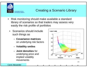
(12) RMOR MSc Lectures in Market Risk Measurement. THE BUSINESS SCHOOL FOR FINANCIAL MARKETS. Creating a Scenario Library. • Risk monitoring should make available a standard library of scenarios so that traders may assess very easily the risk profile of portfolios • Scenarios should include such things as. Figure 13: Smile surface of the FTSE, De 1. Implied Volatlity 1. – Covariance matrices on underlying risk factors. 0.8. – Volatility smiles. 0.4. – Joint densities for underlying price and implied volatility movements. 0.2. 0.6. 0 -0.6. 400 -0.4. -0.2 Moneyness. 0. Carol Alexander. Copyright Carol Alexander, February 2000. 200 0.2 0. Maturity. 23.
(13)
Figure
Related documents