Implicit Syntactic Features for Target dependent Sentiment Analysis

Implicit Syntactic Features for Targeted Sentiment Analysis

Yuze Gao†_{, Yue Zhang}†_{and Tong Xiao}‡ Singapore University of Technology and Design†

Northeastern University‡

yuze gao,yue [email protected] [email protected]

Abstract

Target-dependent sentiment analysis in-vestigates the sentiment polarities on given target mentions from input texts. Dif-ferent from sentence-level sentiment, it offers more fine-grained knowledge on each entity mention. While early work leveraged syntactic information, recent research has used neural representation learning to induce features automatically, thereby avoiding error propagation of syn-tactic parsers, which are particularly se-vere on social media texts.

We study a method to leverage syntac-tic information without explicitly build-ing parser outputs, by trainbuild-ing an encoder-decoder structure parser model on stan-dard syntactic treebanks, and then lever-aging its hidden encoder layers when analysing tweets. Such hidden vectors do not contain explicit syntactic outputs, yet encode rich syntactic features. We use them to augment the inputs to a baseline state-of-the-art target-dependent sentiment classifier, observing signifi-cant improvements on various benchmark datasets. We obtain the best accuracies on two different test sets for targeted senti-ment.

1 Introduction

Target-dependent sentiment analysis investigates the problem of assigning sentiment polarity labels to a set of given target mentions in input sentences. Some example are shown in Table1. For instance, given a sentence “I like [Twitter] better than [ Face-book]”, a target-specific sentiment model is ex-pected to assign a positive (+) sentiment label on

“I like [Twitter]+better thanFacebook”

“I likeTwitterbetter than [Facebook]−”

[lindsay lohan]0goes on yet another emo rant on

her twitter.

Choose [NBI]+for insulation, home energy

au-dits, housing repairing, air sealing, windows and doors,furnaces, air conditioners and en energy efficient appliances.

Table 1: Target-dependent sentiment analysis

w1 w2 w3 w4 w5 w6 w7 w8 w9 w10 w11 w12 w13 w14

Left Context Target Right Context

⊕

- + 0

Figure 1: Sentence level context

the targetTwitterand a negative (−) sentiment la-bel on the targetFacebook.

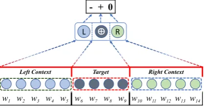
The task has been addressed using neural net-work models, which learn target-specific represen-tations of the input sentence. These representa-tions are then used for predicting target-dependent sentiment polarities. In particular, Dong et al. (2014) derive the syntactic structure of input sen-tence using a dependency grammar, before trans-forming the tree structure to a target-centered form. A recursive neural network is used to trans-form the dependency syntax of a sentence into a target-specific vector for sentiment classification. More recently Vo and Zhang(2015) split the in-put sentence into three segments, with the target entity mention being in the center, and its left and right contexts surrounding it, as shown in Figure1.

x_b

Hidden Vectors fb

(Implicit Syntax)

xt* xt

Top sentiment Model

Input [we_b; we_t; pos_b] Bottomsyntactic Model

Figure 2: Model structure

Rich word embedding features are extracted from the target entity mention and its contexts, which are then used for classification by a linear SVM model. Without using syntactic information, this model gives better accuracies compared with the method ofDong et al.(2014).

Since syntactic parsing of tweets can be inac-curate due to intrinsic noise in their writing style, most subsequent work followed Vo and Zhang (2015), avoiding the use of syntactic informa-tion explicitly. Zhang et al. (2016) applied a bi-directional Gated RNN to learn a dense represen-tation of the input sentence, and then use a three-way gated network structure to integrate target en-tity mention and its left and right contexts. The final resulting representation is used for softmax classification. Tang et al.(2015) also use a RNN (LSTM) to represent the input sentence, yet di-rectly integrating the target embedding to each hidden state for deriving a target-specific vector, which is used for sentiment classification.Liu and Zhang (2017) extended both Zhang et al. (2016) andTang et al.(2015) by introducing the attention mechanism, obtaining the best accuracies on both datasets so far.

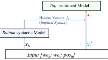
Intuitively, syntactic information should be useful for sentiment analysis given a target, since target-related semantic information such as predicate-argument structure information is con-tained in syntactic structures. The main issue of Dong et al. (2014)’s method is that explicit syn-tactic structures are inaccurate and noisy. We try to avoid this issue by using implicit syntactic in-formation, by integrating the hidden feature layers of a state-of-the-art neural dependency parsing as features to the state-of-the-art targeted sentiment classification models ofLiu and Zhang(2017), us-ing neural stackus-ing (Zhang and Weiss 2016;Chen et al. 2016). The main structure of our model is shown in Figure2.

We choose the parser of Dozat and Manning

(2016) as our syntactic model, which gives the best results on a WSJ benchmark by using multi-layer LSTMs to encode rich input information. The structure of the model is shown in Figure4, which first learns a vector form of each input word (WandT), and then uses a simple bi-affine atten-tion mechanism to find word-word relaatten-tions. The feature vectors (A andD) thus contain rich syn-tactic information about each word, yet do not ex-plicitly specify the syntactic structure of the sen-tence. Hence, using them as features gives our model more syntactic background of the sentence, yet without suffering from error propagation.

Results on both the dataset of Zhang et al. (2016) and the dataset ofTang et al.(2015) show that syntactic information is highly useful for im-proving the accuracies of target-dependent senti-ment analysis. Our final models give the best re-ported results on both datasets. The source code is released at https://github.com/CooDL/

TSSSF.

2 Model

As shown in Figure2, our neural stacking model consists of two brief components: a bottom level syntactic model for obtaining the syntactic infor-mation and a top level sentiment model for target-dependent sentiment classification.

2.1 Input representation

Given an input sentence, we first obtain its word representations. In particular, we train two sep-arate word embedding sets for the bottom level syntactic model and top level sentiment model, re-spectively, denoted as web andwet, respectively.

This is because our syntactic parser is trained on news data, while our sentiment classification is trained on Twitter data.

In addition, for the bottom syntactic model, we also use optionally part-of-speech tag embeddings posb, which are randomly initialised and learned

during the training of the model. Formally, given a wordw, the representation for the bottom level model is:

xb =web⊕posb,

and the input form of the top level model is

xt=x∗t⊕fb=wet⊕Bottom(xb)

Here we use Bottom(xb) indicate the bottom

w1

bilstm layers

w₂ w_n-1 w_n

…

…

…

…

…

…

t₁ t₂ t_n-1 t_n

l1 l2 ln-1 ln

h₁

x1

h₂

x2

h_n-1

xn-1

h_n

xn

… tags …

Figure 3: POS-tagging model

2.2 Syntactic Sub Models

The twitter data suffer poor accuracies by syntax parsers in contrast with news data such as PTB. Directly using explicit twitter syntax features has an error propagation problem. We use a pre-trained syntax model to turn raw word embeddings into implicit syntactic features. Both a POS model and a dependency model are used to utilize syntax features.

2.2.1 POS Model

We employ a simplified bi-directional LSTM (BiLSTM) POS-tagging model (see Figure 3), trained on PTB3 (Toutanova et al. 2003; Labeau et al. 2015). As for every sentence sequence w1, w2, ..., wn, its corresponding word embedding

sequence x1, x2, ..., xn, we integrate its word

embedding into ak1-layer BiLSTM:

S0 _{= [h1, h2, ..., hn]}

= BiLSTM([x1, x2, ..., xn])k1, (1)

where S0 _{is the k1-layer BiLSTM hidden}

state output. A classifier is then used to weight the hidden state of each word inS0 _{and derive the}

la-bel. HereW1is the weight matrix andbis the bias:

Labels= Classifier(W1S0+b), (2)

The BiLSTM hidden layer h1, h2, ..., hn and

the result ofW1S0+b(the labels’ logits) will act as our implicit syntactic features.

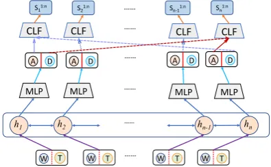
2.2.2 Dependency Model

In this model, we use a dependency parser to re-place the POS-tagging model in Section 2.2.1. In particular, the model of Dozat and Manning (2016) is used, which fuses several BiLSTM lay-ers to encode the input sentence before doing

W T W T …… W T W T

……

h1 h2 hn-1 hn

MLP MLP …… MLP MLP

A D A D A D A D

CLF CLF …… CLF CLF

……

S11:n S21:n …… Sn-11:n Sn1:n

Figure 4: Dependency parsing model

bi-affine attention to learn dependency arcs be-twtween different words.

Two different dependency models are trained: one being a POS⊕ dependency with bottom inputweb⊕posb, one being no-POS dependency

model with just word embedding web. , given

a sentence sequence w1, w2, ..., wn, it integrates

the word embedding web(W) and POS-tag

embedding posb(T) into a k2-layer BiLSTM and generate the LSTM states S0 _{of the words}

in sentenceS, herexi =wei_b⊕posi_b,hi =←h−i⊕−→hi,

S0 _{= [h1, h2, ..., hn]}

= BiLSTM([x1, x2, ..., xn])k2, (3)

MLP (Multilayer Perceptron) layers are used to reduce the dimension size and build features from the BiLSTM state output S0_{. Here it gives four}

kind features:headarc,headdep,relarc,reldep:

headarc, headdep, relarc, reldep

= MLP([h1, h2, ..., hn])k3, (4)

Based on the features, a bi-affine classifier gives every word in the sentence S a corresponding dependency head using the feature headarc(A)

andheaddep(D). We obtain the head relation set

S_head0 ={headj_i, i, j∈[1, n]}:

headj_i = Classifier(headi

arc, headjdep) (5)

Another bi-affine classifier is used to clas-sify the dependency relation based on the feature headarc(A), headdep(D) and headji,

and we obtain the rel relation label set S_rel0 ={relj_i, i, j∈[1, n]}:

b w b w …… b w …… b w …… b w b w

h1 h2 ht1 htm hn-1 hn

⊕ ⊕ ht ⊕ ⊕

h1 h2 …… hn-1 hn

α1 α2 …… αn-1 αn

Sα’

⦿ ⦿

⦿ ⦿

Classifier _P

Figure 5: Target-dependent sentiment analysis with attention, shadow parts donate the attention part in a sentence

Using the two classifiers, we obtain the depen-dency root and relation between every two words in the sentence S. We pre-train the dependency parser model with 4 bi-directional LSTM layers and 2 layers of MLP, and use its intermediate out-put (the MLP outout-put vector) as implicit syntactic feature inputs to the top sentiment model.

The normal dependency syntax model shares the same network frame with the no-POS depen-dency model. They have slight differences in the classifier. Both models are end-to-end denpen-dency parsers with different initial inputs. We choose the same output (Bi-LSTM hidden vector and MLP vector) of the two models as implicit syntactic features.

2.3 Target-dependent Sentiment Model

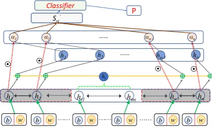
We use the attention-based model of Liu and Zhang(2017) as our top level model. The overall structure is shown in Figure5. Given a sentence, it first uses several BiLSTM layers to learn its syntactic features, and then an attention layer is used to select the relative wegihts of the words according to the target entity over the untargeted words in the whole sentence (Bahdanau et al. 2014;Yang et al. 2016). In particular, for a target word, it applies the target word hidden vector to find a weight forevery word (except the target words) in the sentence (see Figure5). The model also uses a BiLSTM to represent the feature layer from bottom syntactic model fb(b) and the

word embedding wet(w) of a word sequence

w1, w2, ..., wnas the hidden vector of each word.

[h1, h2, ..., hn] = BiLSTM([r1, r2, ..., rn])k4,(7)

where ri = fbi ⊕ weit and k4 is the BiLSTM

layer number.

The target phrase words ht1, ht2, ..., htm are

represented as one vector ht( ht ∈/ [h1, hn]). It

is the average of the target phrase words hidden vectors,ht= _m1

m P i=1hti.

We build a vanilla attention model by calcu-lating a weight value αi for each word in the

sentence. The sentenceSthen can be represented as follows:

S0

α = Attention([h1, h2, ..., hn], ht)

= Pn

i=1αihi, (8)

whereαi = exp(βi)/ n P

j=1exp(βj).

The weight scores βi are calculated by using

target representation ht and each word hidden

vector representation in the sentence,

βi=UTtanh(W2·[hi:ht] +b1), (9)

The sentence representation S0

α is used to

predict the probability vector P sentiment labels on target by:

P = Classifier(W3·Sα0 +b2), (10)

2.4 Training

Our training procedure consists of two steps, one being to pre-train the bottom syntactic models, the other being to apply the pre-trained bottom syn-tactic model and train the top sentiment analysis model.

All models are trained by minimizing the sum of cross-entropy loss and aL2regularization loss of all trainable weights∆W.

loss= _n1 Pn

i σ(yi, y

0

i) +λ2||∆W||2, (11)

The model feature inputs (word embeddings, POS-tag embeddings) are the sum of a trainable embedding and a pre-trained (or learned) embed-ding. All the weight matrix will be initialized with an orthogonal loss less than1e−6_.

We choose different intermediate outputs of dif-ferent bottom level syntax models. For POS-tagging model, we use the BiLSTM hidden out-put (lmpos) and POS-tags vector before softmax

Bottom Syntactic Model LSTM Size(dblstm) 300

MLP Size (dmlp) 100

LSTM Layers(POS Model) (k1) 2

LSTM Layers(Dep. Model) (k2) 4

LSTM Dropout Rate (drblstm) 0.6

MLP Layers (k3) 2

MLP Dropout Rate (drmlp) 0.67

Batch Size(bb) 1000

Word Embeddings (dbw) 100

POS Embeddings (dpos) 100

Top Sentiment Model LSTM Size(dtlstm) 200

LSTM Layers(k4) 1

Word Embedding(dtw) 200

Batch Size(bt) 200

LSTM Dropout Rate(drtlstm) 0.5

Same Parameters Word Minimum Occurance 3 Learning Rate(lr) 0.02 Learning Rate Decay Rate(lrspeed) 0.75

Decay Steps(lrdistance) 1500

Random Seed 1314

Train Iterations 30000

Table 2: Hyper-parameters values

the last BiLSTM layer hidden feature(lmdep) and

the MLP layer output (mlpdep) optionally.

3 Experiments

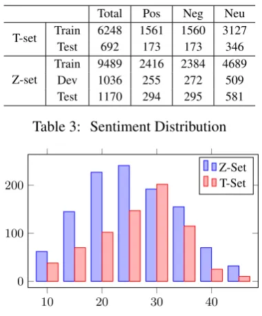
We evaluate the performances of our model and compare them with state-of-the-art results using two standard datasets for target-dependent senti-ment (Zhang et al.,2016;Tang et al.,2015). The PTB3 dataset is used to pre-train our bottom level syntax models.

3.1 Data

We conduct experiments on two datasets, one be-ing the trainbe-ing/dev/test dataset of Zhang et al. (2016) (Z-Set), which consists of the MPQA cor-pus1_{andMitchell et al.(2013)’s corpus}2_{, the other}

being the dataset of the benchmark training/test dataset of?(T-Set), we label these datasets’ POS-tags with the open parser tools ZPar (Zhang and Clark, 2011). Two sets of word embedding are used in this experiment: The GloVe3 ₍

Penning-ton et al., 2014) twitter embedding (100 dimen-sions) for the bottom model, and the GloVe

twit-1_{http://mpqa.cs.pitt.edu/corpora/mpqa corpus/} 2_{http://www.m-mitchell.com/code/index.html} 3_{https://nlp.stanford.edu/projects/glove/}

Total Pos Neg Neu T-set Train 6248 1561 1560 3127

Test 692 173 173 346

Z-set TrainDev 94891036 2416255 2384272 4689509 Test 1170 294 295 581

Table 3: Sentiment Distribution

10 20 30 40

0 100 200

Z-Set T-Set

Figure 6: Test-set length distribution

ter word embedding (200 dimensions) for the top target-dependent sentiment analysis model. Also, due to lack of syntactically labelled twitter data, we used the PTB3 dataset to pre-train our bottom models. We follow the standard splits of PTB3, using 2-21 as the bottom model training data, sec-tion 22 for the development set and 23 as the test set.

We calculate statistics on sentiment polorities and lengths for both datasets. Table 3shows the same percentage of three sentiment labels and Fig-ure6shows length distribution on the test sets.

3.2 Trainning Settings

First, we use the PTB3 dataset with the stan-dard split method pre-train the POS syntax model and dependency syntax model with the hyper-parameters listed in Table2. A best model on the devset is saved for the neural stacking bottom syn-tax model.

Once obtaining the pre-trained bottom syntax model, we build the top sentiment model based on intermediate output syntax model featuresfb and

top word embeddingwet.

3.3 Hyper-parameters

Embedding Size: Our embedding is a

superposi-tion of a trainable and a pre-trained word embed-ding. We fixed the word embedding dimension of webandwetto 100 and 200, respectively to match

Models Acc.(%) F1(%) UAS LAS

POS-tagging 92.4 91.6 / /

Normal Dep. / / 95.6 93.8

No-POS Dep. / / 94.3 92.7

Table 4: Results for Syntactic Sub Model on PTB3 development set.

Dropout Rate: Dropout wrappers are applied to

both the bottom level syntax model and top level sentiment model to avoid overfitting and learn bet-ter features. For the bottom syntax model, we use the PTB3 dataset to pre-train and tune hyper-parameters. A dropout rate of ξ = 0.6 for the BiLSTM layer and a softmax classifier layer to classify the learned features from hidden BiLSTM vector are used, respectively. Dropout rates of ξ = 0.6 andξ = 0.67 are applied to every sec-ond BiLSTM layer and MLP layer, respectively, in the dependency model. We gain the best results (see Table4) of different bottom syntax models on the PTB3 dataset.

For the top sentiment model, we use the model with only top word embedding inputs as our base-line. Here, the bottom syntactic features fb are

pre-processed with a dropout wrapper ofφ= 0.5

before being concatenated to the top model word embedding wet, which is also wrapped with a

dropout ofϕ= 0.8for training models.

Training: We tune the hyper-parameters of the

bottom syntax model on the PTB3 development set and top sentiment on the Z-Set development set. Words that occur less than a minimum amount of 3 times are treated as unknown words. Standard SGD with a decaying learning rate (2e−2_{) is used} for optimization, where the decay rate (0.75) is used to reduce the learning rate after each training iteration step (lrdistance).

lrnew=lr·(lrspeed)totalsteps/lrdistance, (12)

There are several hyper-parameters in our mod-els. We tune all the model hyper-parameters on the dev set with grid-search. With a learning rate ofϕ = 2e−2_{, we did a large parameter iteration} on learning rate decay stepslrdistance, decay rate

lrspeed, batch size (bb&bt) and dropout. The batch

size (bb&bt) has a great impact on model weights

gradient and training speeds, and we choose a balanced point of 200 and 1000 for top and bot-tom model respectively. The decaying learning rate can also help in avoiding early overfitting and

Models Acc.(%)

Baseline 73.24

+lmpos 73.53

+ltpos 73.34

+lmpos&ltpos 73.81

+mlpdep 74.23

+lmdep 73.96

+lmdep&mlpdep 74.59

Table 5: Dev set accuracies for sentiment sub model

Table 6: Dev Results on BiLSTM feature layers

large weights optimization. The details of other hyper-parameters are listed in Table2.

3.4 Development Experiments

Syntactic features:We measure the efficience of different syntax features; the results are listed in Table 5. Within syntactic features, the baseline system (our implementation of Liu and Zhang (2017)) gives an accuracy of 73.24%. With only POS features, the accuracies can reach 74.23%, which is significantly (p < 0.01by T-test) higher. With dependency information, the accuracy further rises to 74.59%, which is significant improved by 1.4 points to the baseline. This shows that syntactic information is indeed useful for target-dependent sentiment classification.

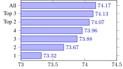
BiLSTM Layers:We also concatenate the hidden

BiLSTM vector from different layers to construct a fast forword feature network to build feature from the dependency model.

lmdep = MLP(CONCAT(lmdep[1 :n])), (13)

here, MLP is used to reduce the concate-nated lmdep dimensions and (1 <= n <= 4).

A dropout wrapper ofφ = 0.6is applied for the concatenated LSTM vectorslmdep[1 :n].

Acc.(%) F1(%) Models Zset Tset Zset Tset

Jiang et al.(2011) / 63.4 / 63.3

Dong et al.(2014) / 66.3 / 65.9

Vo and Zhang(2015) 69.6 71.1 65.6 69.9

Tang et al.(2015) / 71.5 / 69.5

Zhang et al.(2016) 71.9 72.0 69.6 70.9

Liu and Zhang(2017) 73.5 72.4 70.6 70.5 Baseline 73.0 71.7 70.2 70.1

+ lmpos [a] 73.5 72.4 71.2 70.4

+ ltpos [b] 73.2 72.0 70.8 70.2

+ lmpos&ltpos [c] 73.9 72.5 71.4 70.7

+ lmdep 73.5 72.2 70.7 70.6

+ mlpdep 74.0 72.6 71.3 70.9

+ lmdep&mlpdep 74.1 72.7 71.7 71.3

+ lm∗

dep [d] 73.3 72.4 70.9 70.5

+ mlp∗

dep [e] 74.2 72.8 71.3 70.5

+ lm∗

dep&mlp∗dep[f] 74.3 72.8 71.8 71.4

Table 7: Test set results with different syntactic features, the features with∗ _{means they are built}

from the no-POS dependency syntax model

we refer to the first BiLSTM layer as 1, and the

last BiLSTM layer as 4. Top 2 indicates the

layer3 & layer4. Without fast forward connec-tions, the results are 73.24%. With setting 1 to 4, the accuracies increase from 73.24% to 73.32%, 73.67%, 73.88% and 73.96%, respectively. Fi-nally, the best results are obtained with 74.17%. We thus use the settingslayer4for final tests, for a nice balance of efficiency and accuracy.

3.5 Results

We conduct final tests on the test set of Z-Set and T-Set, respectively investigating two ques-tions. First, we verify whether this kind implicit features enhance the accuracy of twitter target-dependent sentiment analysis. Second, we mea-sure how syntax affect target-dependent sentiment analysis results.

First, we compare the effects of different fea-tures on target target-dependent sentiment analy-sis. We take the top model with only word em-bedding inputs as our baseline system. The results are listed in Table 7. We can see that the syntac-tic features contribute to enhancing the accuracy of target-dependent sentiment analysis. Compared with our baseline on both test-set, we obtain an in-crease of Acc. by 1.3 points (p < 0.01) on Z-Set and 1 point (p < 0.05) on T-Set. For the POS-tagging model, the lmpos feature provides more

information than theltposfeature, and theltposhas

Pos Neg Neu

Z-Set BaselineP OS[c] 61.6461.43 69.8370.17 78.6778.97

DEP[f] 61.14 71.14 79.63

T-Set BaselineP OS[c] 62.5761.84 69.3669.41 75.7077.62

DEP[f] 62.74 70.31 78.42

Table 8: F1 values(%) of each polarity on test set of Z-Set, T-Set, theP OS[c]andDEP[f]indicate the features listed in Table7

10 20 30 40

71 72

a b c d e f

Figure 7: Test-set Accuracy against sentence length (Z-Set), a,b,c,d,e,f indicate the features listed in Table7, respectively

little impact in their combination case.

The dependency model features work better than the POS-tag features. lmdep is weaker than

themlpdepfeature, sincemlpdepfeature contains

more learned and special features, which provide the model with sentence level dependency struc-ture.

Second, we separately test the effect of features made with respect to different sentence lengths and sentiment polorities. As two datasets have dif-ferent max sentence lengths (Z-set 84 words, T-set 44 words), we focus on the length range [10,40] and treat the sentence with length 10- and 40+ as 10 and 40, respectively. The results are listed in Table 8, Figure 7 (Here we use the test set of Zhang et al.(2016)). The POS-tags features (a,b,c in Table7) have advantages in short sentence (10-15 words), it gains a significant higher than the dependency features. In contrast, the dependency features (d,e,f in Table7) show larger contribution on longer sentence (30-40 words).

3.6 Analysis

The results show that features have different con-tributions to enhance the accuracy of targeted sen-timent classification. The bottom syntax model output contains different syntactic information. Using them as features do contribution to the top model gain the information about sentence struc-ture or word interrelation.

The POS-tagging model features perform well on short sentences. We believe that a POS-tagging model feature vector contains relation between a present word and its POS context words. This matches its adjacent words, helping model gain lo-cal phrase-level structure information. For exam-ple, if a word has a VB tag and its adjacent words are RB and NN, a tighter relation will be generated between VB and NN.

Phrase-level structure contributes to short sen-tences, but can be ambiguous for long sentence. Even though a RNN can learn some sentence-level information, with the increasing of the sen-tence length, this local benefit can decrease gradu-ally. This can be the reason of the result in Figure 7 where the F1 value of the POS-tagging model drops as the sentence length increase.

The stable performance of the dependency model in Figure 7 suggests that the overall sen-tence structure and local phrase-level structure can be both provided by the dependency model fea-tures. The more nonlocal sentence structure can help the model grasp the sentence sentiment eas-ier. It has a slightly weakened in the overall struc-tures of longer sentence.

The benefits from semantic features is structural and non-sentiment related. Though POS-tag infor-mation can generate dependency relations, we use the PTB3 data to pre-train the bottom level mod-els, where noise may weaken the advantages. In contrast, the dependency model contains more de-tailed information, and is useful for PTB-like for-mal data. The effect can be discounted on twitter data. The results from Table8 show that the F1 values show no significant variation on different sentiment polarities.

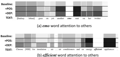
3.7 Attention values

We compared both types of features with the base-line on the attention values and structural relation between words (Figure 8). The relation is com-puted by the top model LSTM hidden vector un-der feature [f] in Table 7. The grey level

cor-[lindsay lohan] goes on yet another emo rant on her twitter .

Baseline:

Choose [NBI] for insulation , air … air conditioners and en energyefficient appliances .

Baseline: +POS: +DEP: TEXT:

(a)emoword attention to others

(b)efficientword attention to others

Figure 8: Word attention under implicit syntactic features, darker grayscale means closer attention

responds to their attention values. Darker colors mean closer attention. Here the baseline is the top model with only word embedding inputs. Figure 8(a) is a short sentence (12 words). We can see that the different features do not affect the sentence structure significantly. The POS-tagging model features focus on its adjacent and related words, such as the word ‘emo’, which has a tight relation with the adjacent word ‘rant’ and its adjunct word ‘another’. When the sentence length increases, the difference between POS and DEP becomes obvi-ous. In Figure 8(b), the DEP has more related darker grey words attention compared to a nor-mal word in the sentence (20+ words, we here hide some words due to limited space). For the phrase ‘en engery efficient appliances’, for exam-ple, the POS features give shallow local relations, but deep remote semantic relations are given by the DEP features, such as the nominal modifier word ‘Choose’ and its paralleling structure word ‘insulation’.

4 Conclusion

the accuracies of the baseline model, and our final model outperforms existing methods that use ex-plicit syntactic features and without syntactic fea-tures, giving the best accuracies on both datasets.

Acknowledgement

We thank the anonymous reviewers for their de-tailed and constructive comments. Yue Zhang is the corresponding author.

References

Dzmitry Bahdanau, Kyunghyun Cho, and Yoshua Ben-gio. 2014. Neural machine translation by jointly

learning to align and translate. arXiv preprint

arXiv:1409.0473.

Hongshen Chen, Yue Zhang, and Qun

Liu. 2016. Neural network for

het-erogeneous annotations pages 731–741.

https://www.aclweb.org/anthology/D/D16/D16-1070.pdf.

Li Dong, Furu Wei, Chuanqi Tan, Duyu Tang, Ming Zhou, and Ke Xu. 2014. Adaptive recursive neural network for target-dependent twitter sentiment clas-sification. InACL (2). pages 49–54.

Timothy Dozat and Christopher D Manning. 2016. Deep biaffine attention for neural dependency

pars-ing. arXiv preprint arXiv:1611.01734.

Long Jiang, Mo Yu, Ming Zhou, Xiaohua Liu, and Tiejun Zhao. 2011. Target-dependent twitter senti-ment classification. InProceedings of the 49th An-nual Meeting of the Association for Computational Linguistics: Human Language Technologies-Volume 1. Association for Computational Linguistics, pages 151–160.

Matthieu Labeau, Kevin L¨oser, Alexandre Allauzen, and Rue John von Neumann. 2015. Non-lexical neural architecture for fine-grained pos tagging. In EMNLP. pages 232–237.

Jiangming Liu and Yue Zhang. 2017. Attention

mod-eling for targeted sentiment. EACL 2017page 572.

Margaret Mitchell, Jacqueline Aguilar, Theresa Wil-son, and Benjamin Van Durme. 2013. Open domain

targeted sentiment. InEMNLP 2013. pages 1643–

1654.

Jeffrey Pennington, Richard Socher, and Christopher D Manning. 2014. Glove: Global vectors for word

representation. InEMNLP. volume 14, pages 1532–

1543.

Duyu Tang, Bing Qin, Xiaocheng Feng, and Ting Liu. 2015. Effective lstms for target-dependent

senti-ment classification. InCOLING. pages 3298–3307.

Kristina Toutanova, Mark Mitchell, and Christopher D Manning. 2003. Optimizing local probability mod-els for statistical parsing.Lecture notes in computer

sciencepages 409–420.

Duy-Tin Vo and Yue Zhang. 2015. Target-dependent twitter sentiment classification with rich automatic

features. InIJCAI. pages 1347–1353.

Zichao Yang, Diyi Yang, Chris Dyer, Xiaodong He, Alex Smola, and Eduard Hovy. 2016. Hierarchical attention networks for document classification. In NAACL-HLT. pages 1480–1489.

Meishan Zhang, Yue Zhang, and Duy-Tin Vo. 2016. Gated neural networks for targeted sentiment

analy-sis. InAAAI. pages 3087–3093.

Yuan Zhang and David Weiss. 2016.

Stack-propagation: Improved representation learning for syntax.arXiv preprint arXiv:1603.06598.

Yue Zhang and Stephen Clark. 2011. Syntactic pro-cessing using the generalized perceptron and beam