On Modeling Sense Relatedness in Multi-prototype Word Embedding
Yixin Cao and Juanzi Li∗and Jiaxin Shi and Zhiyuan Liu and Chengjiang Li Dept. of Computer Science and Technology, Tsinghua University, China 100084
{cao-yx13,ljz,shi-jx,liuzy,licj17}@mail.tsinghua.edu.cn
Abstract
To enhance the expression ability of distributional word representation learn-ing model, many researchers tend to in-duce word senses through clustering, and learn multiple embedding vectors for each word, namely multi-prototype word em-bedding model. However, most related work ignores the relatedness among word senses which actually plays an impor-tant role. In this paper, we propose a novel approach to capture word sense re-latedness in multi-prototype word embed-ding model. Particularly, we differenti-ate the original sense and extended senses of a word by introducing their global oc-currence information and model their re-latedness through the local textual con-text information. Based on the idea of fuzzy clustering, we introduce a ran-dom process to integrate these two types of senses and design two non-parametric methods for word sense induction. To make our model more scalable and ef-ficient, we use an online joint learning framework extended from the Skip-gram model. The experimental results demon-strate that our model outperforms both conventional single-prototype embedding models and other multi-prototype embed-ding models, and achieves more stable performance when trained on smaller data. 1 Introduction
Word embedding, representing words in a low di-mentional vector space, plays an increasing im-portant role in various IR and NLP related tasks, such as language modeling (Bengio et al., 2006;
∗
Corresponding author.
Mnih and Hinton, 2009), named entity recog-nition and disambiguation (Turian et al., 2010;
[image:1.595.309.525.397.486.2]Collobert et al., 2011), and syntactic parsing (Socher et al., 2011, 2013). This trend has been accelerated by the CBOW and the Skip-gram models of (Mikolov et al., 2013b,a) due to its efficiency and remarkable semantic composi-tionality of embedding vectors (e.g. vec(king)-vec(queen)=vec(man)-vec(woman)). However, the assumption that each word is represented by only one single vector is problematic when deal-ing with the polysemous words.
Figure 1: Relatedness among senses of the word “book”.
To enhance the expression ability of the embed-ding model, recent research has a rising enthusi-asm for representing words at sense level. That is, an individual word is represented as multiple vectors, where each vector corresponds to one of its meanings. Pervious work mostly focus on us-ing clusterus-ing to induce word senses (each clus-ter refers to one of the senses) and then learn the word sense representations respectively (Reisinger and Mooney,2010;Huang et al.,2012;Tian et al.,
2014;Neelakantan et al., 2014; Li and Jurafsky,
2015). However, the above approaches ignore the relatedness among the word senses. Hence the fol-lowing limitations arise in the usage of hard clus-tering. First of all, many clustering errors will be caused by using hard clustering based method because the senses of the polysemous word
ally have no distinct semantic boundary (Liu et al.,
2015). Secondly, due to dividing the occurrences of a word into separate clusters, the embedding model will suffer from more data sparsity issue as compared to the Skip-gram model. Thirdly, the embedding quality is considerably sensitive to the clustering results due to the isolation of different sense clusters.
To address this problem, we learn the embed-ding vectors of the word senses with some com-mon features if the senses are related. Instead of clearly cutting the sense cluster boundaries, one occurrence of the word will be assigned into multiple sense clusters with different probabili-ties, which agrees with a classic task of word sense annotation, Graded Word Sense Assignment (Erk and McCarthy,2009;Jurgens and Klapaftis,
2013).
Actually, the senses of a polysemous word are related not only by the contiguity of mean-ing within a semantic field1, but also by the ex-tended relationship between the original meaning and the extended meaning (Von Engelhardt and Zimmermann, 1988). We investigate the relat-edness of the synsets (word senses) in WordNet (Miller, 1995) through the Wu & Palmer mea-sure2 (Wu and Palmer,1994), and present an in-teresting example of the word “book” in Figure
1. The right side is the similarity matrix of its 11 nominal synsets, wheresi denotes theith synset.
Each tile represents a similarity value between two synsets whose color deepens as the value in-creases. The left side is their frequencies in Word-Net. On one hand, we can see apparent correla-tions among these senses in different levels. Note that (s1, s2, s11) are strongly related, and so are
(s6, s7)and(s8, s9, s10). This is because of their extended relationship. Take (s1, s2, s11) for ex-ample,s1 refers to the sense of “the written work
printed on pages bound together”, s2 refers to “physical objects consisting of a number of pages bound together” and s3 refers to “a number of
sheets (or stamps, etc.) bound together”. Obvi-ously, s1 is the original meaning, s2 and s11 are the extended meanings. Moreover, the relatedness suggests that the senses share some common tex-tual features in the contexts. On the other hand, the frequency of the original meanings1 is much
1According to https://en.wikipedia.org/wiki/Polysemy. 2The Wu & Palmer measure is an edge based approach
that is tied to the structure of WordNet. Also, one can try different relatedness approaches and will find similar results.
higher than that of the extended meaningss2 and
s11, which suggests that the word sense distribu-tion in corpus should be taken into account when modeling word sense relatedness.
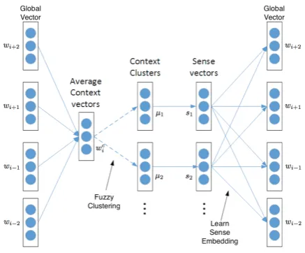
[image:2.595.307.526.372.553.2]In this paper, we propose a novel method, namely FCSE (Fuzzy Clustering-based multi-Sense Embedding model), that models the relat-edness among word senses by using the fuzzy clustering based method for word sense induc-tion, and then learns sense embeddings via a vari-ant of Skip-gram model. The basic idea behind fuzzy clustering is that the senses may be related and share common features through the overlaps of the sense clusters. Based on our observations of the original meaning and the extended mean-ing, we further design two non-parametric meth-ods, FCSE-1 and FCSE-2, to model the local textual context information of senses as well as their global occurrence distribution by incorporat-ing the Generalized Polya Urn (GPU) model. For efficiency and scalability, our proposed model also adopts an online joint learning procedure.
Figure 2: Framework of FCSE
2 The Framework of FCSE
FCSE adopts an online procedure that induces the word sense and learns the sense embed-dings jointly. Given a word sequence D =
{w1, w2, . . . , wM}, we obtain the input of our
model, the word and its context words, by sliding a window with the length of2k+ 1. The output is also the context words. During the learning pro-cess, two types of vectors are maintained for each word, the global vectorwi and its sense vectors3
wsi
i . Note that the number of senses|Si|is
vary-ing because the cluster method is non-parametric. As shown in Figure 2, there are mainly two steps: the clustering step and the embedding learn-ing step. The former step incrementally clus-ters all the occurrences of one word according to its context vectors by computing the average sum of the global vectors of the context words:
wc
i = 21k
P
−k≤j≤kwi+j. Each cluster refers to one word sense, thus each occurrence will be an-notated with at least one sense.
In the second step, we update the sense em-beddings via a variant of the Skip-gram model (Mikolov et al., 2013b). The main difference be-tween our model and Skip-gram is that we aim to predict the context words given the exact sense of the target word instead of the word itself. More-over, because several senses are assigned to the current word with probabilities, we leverage all the related senses to predict the context words. The intuition is that the related senses tend to have common context words as mentioned in Section
1. Thus, all the assigned sense vectors will be up-dated with weights simultaneously as follows:
L(D) = M1 M
X
i=1
X
−k≤j≤k |Si|
X
si
λsilogp(wi+j|wisi)
(1) where the probability of p(wi+j|wisi) is defined
using softmax function, and si denotes the sense
index of wordwi. Siis the set of existing senses,
λsiis the update weight of sense si. We set the weights proportional to the probabilities of the current word being annotated with sensesi, which
is equivalent to the results of fuzzy clustering, the likelihood of the contextwc
i assigned into the
sense clustersi:
λsi ∝
p(si|wci) siis sampled
0 otherwise (2)
Finally, we use negative sampling technique4for efficient learning.
3 Word Sense Induction
Section 2 describes the framework of our model including how to obtain the input features of clus-tering and to use the cluster results for the sense 4More detailed information can be found in (Mikolov et al.,2013b).
embedding learning. In this section, we present two fuzzy clustering based methods for clustering-based word sense induction, FCSE-1 and FCSE-2. Both of them are nparametric and conduct on-line procedures.
Based on our observations in Section1, the oc-currence of word senses is usually distinguishing between the original meaning and the extended meaning, while the original meaning and its ex-tended meanings are semantically related with some common textual contexts. Considering both of the two aspects, in FCSE-1, we induce the word sense according to the cluster probability propor-tional to the distance of its centroid to the cur-rent word’s contexts; and FCSE-2 utilizes a ran-dom process, the Generalized Polya Urn (GPU) model, to further incorporate the senses’ global occurrence distribution.
3.1 FCSE-1
Adopting an online procedure, FCSE-1 clusters the contexts of one word incrementally. When first meet one word, we create a cluster with the centroid of its context vector. Then, for each oc-currence of the word, several existing clusters are sampled following a probability distribution; or a new cluster is created only if all the probabili-ties of the context belonging to the clusters equal to zero. Finally, all the sampled clusters will be updated by adding the current context vector into them.
Remember that each wordwiis associated with
a global vector, varying number of clusters, and the corresponding sense vectors. FCSE-1 mea-sures the semantic distance of the context vector to its cluster centers, and aims to sample the near-est ones (maybe multiple related senses). Given the context vectorwc
i, the probability of the word
belonging to the existinglth sense is:
p(si =l|wci) =
1
ZSim(µli, wic) 0 if Sim(µl
i, wci)< under
(3) where µl
i denotes the centroid of thelth sense
cluster,Z is the normalization term andSim(·,·)
can be any similarity measurement. In the experi-ments we use cosine similarity as the semantic dis-tance measurement.underis a pre-defined
thresh-old that indicates how easily we create a new sense cluster. Similarly, we use another thresholdupper
Sup-pose that the probabilities{pni|ni ∈Si}is ranked in descending order, then we pick up the clus-ters with topni probabilities untilpni−pni+1 >
upper. Note that the hyper-parameters meet0 ≤
under, upper≤1.
3.2 FCSE-2
Since FCSE-1 uses two hyper-parameters to re-spectively control a new cluster initialization and the number of clusters sampled, which is difficult to set manually. So, instead of the fixed thresholds, we make a further randomization by introducing a random process, GPU, in FCSE-2. Besides, more inherit properties of the word senses can be taken into account, including not only the local informa-tion of the semantic distance from the context to the cluster centers, but also the frequency, which is related to how likely the current sense is an orig-inal meaning or an extended meanings.
In this section, we will firstly give a brief sum-marization of the GPU model, and then introduce how to incorporate it into our model.
3.2.1 Generalized Polya Urn model
Polya urn model is a type of random process that draws balls from an urn and replaces it along with extra balls. Suppose that there are some balls of colors in the urn at the beginning. For each draw, the ball of theith color is selected followed by the distribution:
p(color=i) = mmi
where m is the total number of balls, and mi is
the number of balls of the ith color. A standard urn model returns the ball back along with an extra ball of the same color, which can be seen as a rein-forcement and sometimes expressed as the richer gets richer. More detailed information can be found in the survey paper (Pemantle et al.,2007). Polya urn model can be used for non-parametric clustering, where each data point refers to a ball in the urn, and its cluster label is denoted by the ball’s color.
Since the fixed replacement lacks of flexibility, the GPU model conducts the reinforcement pro-cess following another distribution over the colors. That is, when a ball of color iis drawn, another
Aij balls of color j will be put back. Then, for
each draw, we replace the ball with different num-ber of balls of various colors according to the dis-tribution matrixA. As repeating this process, the
drawing probability will be altered if the number of extra balls are nonzero.
3.2.2 Incorporating GPU into Embedding model
The induction process of the word senses can be regarded as a GPU model. The original meaning is sampled firstly, and then the extended meanings are sampled through the reinforcement. That is, we sample an extended meaning according to a conditional probability given the original mean-ing. The basic idea is that knowing the original meaning is necessary for understanding the tar-get word annotated with an extended meaning in a document. For example, the extended meaning of the word “milk” when used in the terms “glacier milk” won’t be well understood unless we know the original meaning of “milk”.
Correspondingly, in the GPU model, a urn de-notes a word, the ball and the color refers to the occurrence and the sense, respectively. Note that each ball has an index that distinguishes different occurrences. Thus, the balls of the same color cor-respond to a sense cluster.
We sample the related senses in two stages. In the first stage, for the occurrence of the wordwi,
we sample a sensesio =lconsidering the global
distribution of the word senses as well as the se-mantic distance from the context features to the cluster center. In the second stage, several senses are sampled conditioned on the previous result:
p(sie =l0|sio=l).
In this way, we find the original meaning and the extended meanings separately following dif-ferent distributions. Considering the observation that the original meaning occurs more frequently (as described in Section1), we define the probabil-ity distribution of the original meaning as follows:
p(sio =l|wci)∝
( m
il
γ+mi ·Sim(µ
l
i, wci) l∈Si γ
γ+mi l is new (4) wheremi is the total number of occurrences of
the target word wi, mil is the number of the lth
cluster and we havePSi
l mil=mi. Note thatγis
a hyper-parameter that indicates how likely a new cluster will be created, and its impact decreases as the size of training datamiincreases.
fea-tures as well as the cluster center sampled in the first stage, which is defined as follows:
p(sie =l0|sio=l, wic)∝e·Sim(wsiie,w sio
i +wci
2 )
(5) where e varies from 0 to 1 and controls the
strength of the reinforcement. We will talk about it in the next subsection.
Sampling separately, the relatedness of the orig-inal meaning and the extended meanings are mod-eled and each occurrence of the word has been annotated with one original sense and several ex-tended senses (or there is no additional exex-tended meanings). Note that the likelihood of the oc-currence of the word annotated with an extended meaning isp(sie = l0|sio = l, wic)p(sio = l|wic).
Clearly, the probabilities of sampling the extended meanings are always lower than that of the origi-nal meaning.
3.3 Relationship with State-of-the-art Methods
FCSE-1 The hyper-parameters meet 0 ≤
under, upper ≤ 1. upper is used to control the
number of clusters assigned to the current word, and FCSE-1 will degrade to hard assignment if we setupper = 0, which is similar with the
NP-MSSG model in (Neelakantan et al., 2014). We can useunderto control the sense number of each
word, and an extreme case ofunder = 0denotes
that we create only a sense cluster for each word, then the model is equivalent to the Skip-gram.
FCSE-2 The number of the extended meanings |Sie|varies from 0 to |Si−l|, where S−i l denotes
the set excluding the original meaning sl i. The
hyper-parameter 0 ≤ e ≤ 1 is used to control
the strength of the GPU reinforcement as well as the number of the extended meanings. Particu-larly, if we set e = 0, the second sample for
the extended meanings has been turned off, and then FCSE-2 degrades to the SG+ model in (Li and Jurafsky,2015), which is another state-of-the-art method for multi-prototype word embedding model based on hard clustering. By settingγ = 0
in Equation4, which is used to control the proba-bility of creating a new sense, FCSE-2 won’t cre-ate new senses. Learning a single sense for each word makes the step of sense sampling becomes meaningless. Thus, FCSE-2 uses the only em-bedding of the current word to predict its context
words, which is equivalent to the Skip-gram.
4 Empirical Evaluation
In this section, we demonstrate the effectiveness of our model from two aspects, qualitative and quantitative analysis. For qualitative analysis, we presents nearest 10 neighbors for each word sense to give an intuitive impression. For quantitative analysis, we conduct a series of experiments on the NLP task of word similarity using two bench-mark datasets, and explore the influence of the size of training corpus.
4.1 Data Preparation
We train our model on Wikipedia, the April 2010 dump also used by (Huang et al.,2012;Liu et al.,
2015;Neelakantan et al., 2014). Before training, we have conducted a series of preprocessing steps. At first, the articles have been splitted into sen-tences, following by stemming and lemmatization using the python package of NLTK5. Then, we rank the vocabulary according to their frequencies, and only learn the embeddings of the top 200,000 words. The other words out of the vocabulary are replaced by a pre-defined mark “UNK”. Note that FCSE is slower than word2vec6, but the efficiency is far away from being an obstacle on training.
Below we describe three baseline methods and parameter settings, followed by qualitative anal-ysis of nearest neighbors of each word sense. Then, quantitative performance will be presented via experiments on two benchmark word similar-ity tasks.
4.2 Baseline Methods
Word Embedding model can be roughly divided into two types: single vector embedding model and multi-prototype embedding model. To vali-date the performance, we compare our model with three models of both the two types: Skip-gram, NP-MSSG and SG+. The reason why we select them as the baseline methods is because: (i) they are the state-of-the-art methods of word embed-ding model; (ii) NP-MSSG and SG+ adopts the similar learning framework to our model.
• Skip-gram∗ aims to leverage the current
word to predict the context words and learn 5http://www.nltk.org/
6https://code.google.com/archive/p/
Apple
Skip-gram∗ iigs, boysenberry, apricot, nectarine, ibook, ipad, blackberry, blackcurrants,
loganberry, macintosh
NP-MSSG∗ nectarine, boysenberry, peach, blackcurrants, pear, passionfruit, feijoa,
lo-ganberry, elderflower, apricot
macintosh, mac, iigs, macworks, macwrite, bundled, compatible, laser-writer, ibook, ipod
FCSE-1 nectarine, blackcurrants, loganberry, pear, boysenberry, strawberry, apricot,plum, cherry, blueberry macintosh, imac, iigs, ibook, ipod, pcpaint, iphone, booter, ipad, macbook Berry
Skip-gram∗ greengage, thimbleberry, loganberry, dewberry, boysenberry, pome,
pas-sionfruit, acai, maybellene, blackcurrant
NP-MSSG∗ thimbleberry, pome, nectarine, greengage, fruit, boysenberry, dewberry,
acai, loganberry, ripe
[image:6.595.96.506.70.326.2]FCSE-1 nectarine, thimbleberry, blueberry, fruit, pome, loganberry, apple, elder-berry, passionfruit, litchi gordy, taylor, lambert, osborne, satchell, earland, thornton, fullwood, allen, sherrell
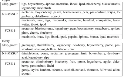
Table 1: Nearest 10 neighbors of each sense of the words “apple” and “berry”, computed by cosine similarity, for different models.
the embeddings within a two-layer neural network.
• NP-MSSG∗measures the distance of the
cur-rent word to each sense, picks up the nearest one and learning its embedding via a standard Skip-gram model.
• SG+∗ improves the NP-MSSG model by
in-troducing a random process that induces the word sense with probabilities.
The symbol∗denotes that we, instead of using their released codes, carefully reimplement these models for the sake of making the comparisons as fairly as possible. Thus, all the models share the same program switched by the correspondingly parameters (as described in Section3.3). Note that there may be some minor differences such as op-timizing tricks between our program and that of their released.
4.3 Parameter Setting
As discussed in Section 3.3, our model can de-grade to the baseline methods by switching dif-ferent parameters: the thresholdupper,eand the
max number of word sensesNMAX. All the
meth-ods are implemented on the same java program7, and use, at the greatest extent, the same settings in-cluding the training corpus, shared parameters and the program code, etc.
Switching parameters For FCSE-1 and NP-MSSG,upperis set 0.05 and 0, respectively.
Sim-ilarly, We sete = 1for FCSE-2, ande = 0for
SG+. When setting NMAX = 1, all the
multi-prototype word embedding models degrade to sin-gle vector embedding model, that is, the Skip-gram model.
Shared parameters Following the original pa-pers of NP-MSSG and SG+, the thresholdunder
in FCSE-1 is also set with -0.5, andγ = 0.01is used in both FCSE-2 and SG+. The initial learn-ing rateα = 0.015is used for parameter estima-tion. We pick up 5 words as the context window, and 400 dimensional vectors to learn sense embed-dings of the top 200,000 frequent words. Note that all the parameters including the embedding vec-tors are initialized randomly.
7We will publish the code if accepted, which
4.4 Qualitative Analysis
Before conducting the experiments on word simi-larity task, we first give qualitative analysis of our model as well as two baseline models8 by repre-senting the word sense with its nearest neighbors, which are computed through cosine similarity of the embeddings between each of the word senses and the senses of the other words.
Table 1 presents the nearest 10 neighbors of each sense of two words ranked through the sim-ilarity. Skip-gram shows a mixed result of differ-ent senses, while the other two models produce a reasonable number of word sense, and their neigh-bors are indeed semantically correlated. For the word “Apple”, there are two meanings of the fruit and technology company. NP-MSSG and FCSE-1 can differentiate the two senses, but FCSE-FCSE-1 clearly achieves a more coherent ranking results. For the word “Berry”, FCSE-1 outperforms NP-MSSG for it successfully identifies another sense of person’s name except the dominant sense of fruit. This is because “Berry” is used as a person’s name much less frequently than a fruit. Thus, it may cause the data sparsity issue, while our model is capable of addressing this problem by improv-ing the usage of trainimprov-ing corpus, which will be fur-ther discussed in Section4.5.3.
4.5 Word Similarity
In this subsection, we evaluate our embeddings on two classic tasks of measuring word similarity: word similarity and contextual word similarity. To better test the ability of our model to address the problem of data sparsity, we train it using only 30% of the training corpus (sampled randomly). Also, we give comparisons with the performance using all the training data.
WordSim353 (Finkelstein et al., 2001) is a benchmark dataset for word similarity. It contains 353 word pairs and their similarity scores assessed by 16 subjects. SCWS, released by (Huang et al.,
2012), is a benchmark dataset for contextual word similarity, which computes the semantic related-ness between two words conditioned on the spe-cific context. It consists 2,003 pairs of words and their sentential contexts. WordSim353 focuses on the ambiguity among similar words, and SCWS is for the ambiguity of word senses in different con-8To be fair, we only show the comparisons among
FCSE-1, NP-MSSG and Skip-gram, since the paper of SG+ (Li and Jurafsky,2015) didn’t give the qualitative results.
texts.
4.5.1 Evaluation Metrics
To evaluate the performance of our model, we compute the similarity between each word pair through some measurement, and then use the spearman correlation between our results and the human judgments to evaluate the performance of the model.
Working on WordSim353, we compute the average similarity between the word pairs the same as(Reisinger and Mooney,2010; Neelakan-tan et al., 2014). And working on SCWS, we use two similarity measurements, avgSimC and maxSimC, proposed by (Neelakantan et al.,2014;
Liu et al.,2015). avgSimC focuses on evaluating the average similarity between all the senses of the two words, and maxSimC evaluates the similarity between the senses with max probability for the current word.
4.5.2 Results and Analysis
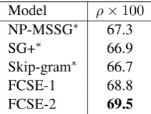
Table 2 and 3 shows the overall performance of our proposed model as well as the baseline meth-ods on WordSim353 and SCWS datasets. We only obtain lower performance numbers for SG+, which suggests that they may be more susceptible to noise and worse generalization ability. How-ever, this is a fair comparison because all the meth-ods share the same parameter settings and the code. The following is indicated in the results:
Model ρ×100
NP-MSSG∗ 67.3
SG+∗ 66.9
Skip-gram∗ 66.7
FCSE-1 68.8
FCSE-2 69.5
Table 2: Results on the wordsim353 dataset. The table presents spearman correlation ρ between each model’s similarity rank results and the human judgement.
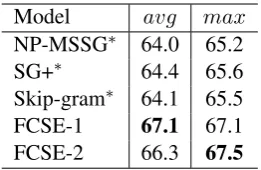
[image:7.595.361.471.493.576.2]Model avg max
NP-MSSG∗ 64.0 65.2
SG+∗ 64.4 65.6
Skip-gram∗ 64.1 65.5
FCSE-1 67.1 67.1
[image:8.595.116.247.61.146.2]FCSE-2 66.3 67.5
Table 3: Results on the SCWS dataset. “avg” and “max” respectively denotes the similarity mea-surements of avgSimC and maxSimC.
• The skip-gram model achieves rather com-parative performance due to its good general-ization ability, especially in a smaller training set as compared to hard-cluster based multi-prototype word embedding models.
• FCSE-2 achieves the best performance due to the separately sample for the original meaning and the extended meanings, which follows different distributions incorporating both the global and local information.
We also investigate the ability of our method that helps address the data sparsity issue by train-ing on different size of data.
4.5.3 Training on Different Size Data
Generally speaking, the embedding model per-forms better when trained on a larger corpus. The multi-prototype embedding model suffers more data sparsity issue than single prototype embed-ding due to its further partition on the set of words’ contexts by clustering, and then performs even worse using a smaller training corpus. In this sub-section, we study the capability of FCSE to helps address this problem by testing the performance when training on different size corpus.
Figure3shows the comparison between the per-formance of all the models trained on 30% data and on 100% data. As the training data decreases, all the models perform worse especially the hard clustering based method. Compared to full cor-pus, we can see more apparent gap between NP-MSSG and FCSE-1 (from 2.6% to 3.1%), SG+ and FCSE-2 (from 0.1% to 1.9%). That is, the gap between FCSE and other methods gets closer when there are adequate training corpus, which is in accordance with the intuition. The data spar-sity issue gradually vanishes along with the growth of training data. Besides, the performance of the single-prototype word embedding model increases
Figure 3: The performance of each model when training on different size of data
only 1.6%. Our proposed model, both FCSE-1 and FCSE-2, achieves more stable performance (0.2% and 0.6% changes).
5 Related Work
Multi-prototype word embedding has been exten-sively studied in the literature (Chen et al.,2014;
Cao et al., 2017;Liu et al., 2015; Reisinger and Mooney, 2010; Huang et al., 2012; Tian et al.,
2014;Neelakantan et al., 2014; Li and Jurafsky,
2015). They can be roughly divided into three groups. The first group is clustering based meth-ods. As described in Section 1, (Reisinger and Mooney, 2010; Huang et al., 2012; Tian et al.,
2014;Neelakantan et al., 2014; Li and Jurafsky,
2015) use clustering to induce word sense and then learn sense embeddings via Skip-gram model. The second group is to introduce topics to represent different word senses, such as (Liu et al., 2015) considers that a word under different topics leads to different meanings, so it embeds both word and topic simultaneously and combines them as the word sense. However, it is difficult to de-termine the number of topics. The third group incorporates external knowledge (i.e. knowledge bases) to induce word/phrase senses. (Chen et al.,
[image:8.595.311.521.61.219.2]6 Conclusion
In this paper, we propose a novel method that models the word sense relatedness in multi-prototype word embedding model. It considers the difference and relatedness between the orig-inal meanings and the extended meanings. Our proposed method adopts an online framework to induce the word sense and learn sense embeddings jointly, which makes our model more scalable and efficient. Two non-parametric methods for fuzzy clustering produce flexible number of word senses. Particularly, FCSE-2 introduces the Gen-eralized Polya Urn process to integrate both the global occurrence information and local textual context information. The qualitative and quantita-tive results demonstrate the stable and higher per-formance of our model.
In the future, we are interested in incorporating external knowledge, such as WordNet, to super-vise the clustering results, and in extending our model to learn more precise sentence and docu-ment embeddings.
7 Acknowledgments
The work is supported by 973 Program (No.
2014CB340504), NSFC key project (No.
6153301861661146007), Fund of Online Educa-tion Research Center, Ministry of EducaEduca-tion (No. 2016ZD102), and THUNUS NExT Co-Lab.
References
Yoshua Bengio, Holger Schwenk, Jean-S´ebastien Sen´ecal, Fr´ederic Morin, and Jean-Luc Gauvain. 2006. Neural probabilistic language models. In
Innovations in Machine Learning, pages 137–186. Springer.
Yixin Cao, Lifu Huang, Heng Ji, Xu Chen, and Juanzi Li. 2017. Bridge text and knowledge by learning multi-prototype entity mention embedding. In Pro-ceedings of the 55th annual meeting of the associ-ation for computassoci-ational linguistics. Association for Computational Linguistics.
Xinxiong Chen, Zhiyuan Liu, and Maosong Sun. 2014. A unified model for word sense representation and disambiguation. InProceedings of the 2014 Con-ference on Empirical Methods in Natural Language Processing (EMNLP), pages 1025–1035.
Ronan Collobert, Jason Weston, L´eon Bottou, Michael Karlen, Koray Kavukcuoglu, and Pavel Kuksa. 2011. Natural language processing (almost) from scratch. The Journal of Machine Learning Re-search, 12:2493–2537.
Katrin Erk and Diana McCarthy. 2009. Graded word sense assignment. InProceedings of the 2009 Con-ference on Empirical Methods in Natural Language Processing: Volume 1-Volume 1, pages 440–449. Association for Computational Linguistics.
Lev Finkelstein, Evgeniy Gabrilovich, Yossi Matias, Ehud Rivlin, Zach Solan, Gadi Wolfman, and Ey-tan Ruppin. 2001. Placing search in context: The concept revisited. InProceedings of the 10th inter-national conference on World Wide Web, pages 406– 414. ACM.
Eric H Huang, Richard Socher, Christopher D Man-ning, and Andrew Y Ng. 2012. Improving word representations via global context and multiple word prototypes. InProceedings of the 50th Annual Meet-ing of the Association for Computational LMeet-inguis- Linguis-tics: Long Papers-Volume 1, pages 873–882. Asso-ciation for Computational Linguistics.
David Jurgens and Ioannis Klapaftis. 2013. Semeval-2013 task 13: Word sense induction for graded and non-graded senses. InSecond joint conference on lexical and computational semantics (* SEM), vol-ume 2, pages 290–299.
Jiwei Li and Dan Jurafsky. 2015. Do multi-sense embeddings improve natural language understand-ing? In Proceedings of the 2015 Conference on Empirical Methods in Natural Language Process-ing, EMNLP 2015, Lisbon, Portugal, September 17-21, 2015, pages 1722–1732.
Yang Liu, Zhiyuan Liu, Tat-Seng Chua, and Maosong Sun. 2015. Topical word embeddings. In Twenty-Ninth AAAI Conference on Artificial Intelligence. Tomas Mikolov, Kai Chen, Greg Corrado, and Jeffrey
Dean. 2013a. Efficient estimation of word represen-tations in vector space.CoRR, abs/1301.3781. Tomas Mikolov, Ilya Sutskever, Kai Chen, Greg S
Cor-rado, and Jeff Dean. 2013b. Distributed representa-tions of words and phrases and their compositional-ity. InAdvances in neural information processing systems, pages 3111–3119.
George A Miller. 1995. Wordnet: a lexical database for english. Communications of the ACM, 38(11):39– 41.
Andriy Mnih and Geoffrey E Hinton. 2009. A scal-able hierarchical distributed language model. In
Advances in neural information processing systems, pages 1081–1088.
Robin Pemantle et al. 2007. A survey of random pro-cesses with reinforcement. Probab. Surv, 4(0):1–79. Joseph Reisinger and Raymond J Mooney. 2010. Multi-prototype vector-space models of word mean-ing. InHuman Language Technologies: The 2010 Annual Conference of the North American Chap-ter of the Association for Computational Linguistics, pages 109–117. Association for Computational Lin-guistics.
Richard Socher, John Bauer, Christopher D Manning, and Andrew Y Ng. 2013. Parsing with composi-tional vector grammars. In In Proceedings of the ACL conference. Citeseer.
Richard Socher, Cliff C Lin, Chris Manning, and An-drew Y Ng. 2011. Parsing natural scenes and natu-ral language with recursive neunatu-ral networks. In Pro-ceedings of the 28th international conference on ma-chine learning (ICML-11), pages 129–136.
Fei Tian, Hanjun Dai, Jiang Bian, Bin Gao, Rui Zhang, Enhong Chen, and Tie-Yan Liu. 2014. A probabilis-tic model for learning multi-prototype word embed-dings. InProceedings of COLING, pages 151–160. Joseph Turian, Lev Ratinov, and Yoshua Bengio. 2010.
Word representations: a simple and general method for semi-supervised learning. InProceedings of the 48th annual meeting of the association for compu-tational linguistics, pages 384–394. Association for Computational Linguistics.
Wolf Von Engelhardt and J¨org Zimmermann. 1988.
Theory of earth science. CUP Archive.