Sliding Mode Control of Descriptor Systems

(1)

Sliding Mode Control of Descriptor Systems

Anusha Rani V1

Assistant Professor, Dept. of EIE, PSN College of Engineering and Technology, Tirunelveli, India

ABSTRACT: This paper concentrates on the work done on sliding mode control of descriptor systems. Any practical control problem there always be a discrepancy between the actual plant and its mathematical model. These discrepancies (or mismatches) mostly come from unknown external disturbances, plant parameters and unmodeled dynamics. Robust properties of the plant with these disturbances are studied with the help of sliding mode control. Non-Linear systems are studied using the sliding mode control. SMC design can be divided into two subparts viz. (1) the design of a stable surface and (2) the design of a control law to force the system states onto the chosen surface in finite time. The design of the surface should address all constraints and required specifications therefore it should be designed optimally to meet all requirements. The values of gain are obtained using several methods and these values are used in the regulation of the SMC. The tracking control is incorporated to the chemical processes.

KEYWORDS: Sliding mode control, Descriptor systems, Robust, Non-Linear systems, unmodeled dynamics.

I.INTRODUCTION

Any practical control problem there always a discrepancy between the actual plant and its mathematical model. These discrepancies (or mismatches) mostly come from unknown external disturbances, plant parameters and modeled dynamics. Robust properties of the plant with these disturbances are studied with the help of sliding mode control. Beginning in the late 1970s and continuing today, the sliding mode control has received plenty of attention due to its insensitivity to disturbances and parameter variations. The well-known sliding mode control is a particular type of Variable Structure. Control System (VSCS). Recently many successful practical applications of sliding mode control (SMC) have established the importance of sliding mode theory which has mainly been developed in the last three decades. This fact is also witnessed by many special issues of learned journals focusing on sliding mode control. The research in this field was initiated by Emel’yanov and his colleagues, and the design paradigm now forms a mature and an established approach for robust control and estimation. The idea of sliding mode control (SMC) was not known to the control community at large until an article published by Utkin and a book by Itkis.

SMC design can be divided into two subparts viz. (1) the design of a stable surface and (2) the design of a control law to force the system states onto the chosen surface in finite time. The design of the surface should address all 2 constraints and required specifications therefore it should be designed optimally to meet all requirements.

The effectiveness of SMC in the robust control of linear uncertain systems prompted the research of sliding mode control in other types of systems. Thus, a few researchers worked on the sliding mode control of nonlinear systems and time delay systems. To relax the need for measuring the entire state vector, an output feedback based sliding mode concept is also proposed in which widens the scope of sliding mode control.

II.NON-LINEAR AND DESCRIPTOR SYSTEMS

A.NON LINEAR SYSTEM

(2)

Generally, nonlinear problems are difficult (if possible) to solve and are less predictable than linear problems. Even if not exactly solvable, the outcome of a linear problem is rather predictable, while the outcome of a nonlinear is inherently not. Hence we choose to implement the non-linear system through the Intelligent Controllers which otherwise is a challenging task. If the controller works for a nonlinear system then it is versatile, which allow us to apply for any other system?

B.DESCRIPTOR SYSTEMS

Descriptor state-space models can include both dynamic and algebraic equations, as is common in electrical circuits or constrained mechanical systems. This makes modeling easier and allows for more general systems. Descriptor system descriptions frequently appear when solving computational problems in the analysis and design of standard linear systems.

Many operations on standard matrices (e.g., finding the rank, determinant, inverse or generalized inverses), or the solution of linear matrix equations can be performed for rational matrices as well using descriptor system techniques. Other important applications of descriptor techniques are the computation of inner-outer and spectral factorizations, or minimum degree and normalized coprime factorizations of polynomial and rational matrices.

SLIDING MODE CONTROL AND LINEAR STATE FEEDBACK

Consider a first order uncertain system modeled as

ẋ(t)=ax(t)+bu(t)+ρ(x,t) (1)

Where x(t)∈ R, u(t) ∈ R, and a,b are known nonzero constants. The term ρ(x, t)∈R accounts for the uncertainty and only the bounds of this uncertain term are known. The control objective is to stabilize x(t) when only the bounds of uncertainty are known. To stabilize the uncertain system in (4), if initial value of x(t) is positive then ẋ(t) should be negative and vice versa. Therefore, depending on the sign of x(t), control law should be altered to ensure stabilization of x(t). Consider a control law:

u(t) = −b−1(ax(t)+Q sign(x)) (2)

Where sign (.) represents the signum function, and Q > 0 is chosen such that

|ρ (x, t)| ≤ Q (3)

With control law (2) system (1) becomes

ẋ(t) = −Q sign(x(t))+ρ (x, t) (4)

To analyze the above closed loop system, consider the case when initial condition x(0)>0. Due to condition (3), it follows that ẋ(t)<0. Therefore, x(t) is decreasing and moving towards x(t) = 0. When initial condition x(0)<0, then using condition (3), it implies that ẋ>0. Therefore x(t)>0 and approaches x(t) = 0.So in this case also x(t) is moving towards the line x(t) = 0. Thus, irrespective of the initial condition, with control law (2), the system state x(t) is forced towards x(t) = 0. The control law ensures a minimum rate of decrease (or increase) of x(t) therefore x(t) reaches in finite time. At x(t)=0, the discontinuous part of the control law is not defined. However, the moment the trajectory crosses x(t) = 0 from either direction, again it is forced back on x(t) = 0. Because the control law is discontinuous about x(t) = 0 it demands switching at very high frequency. If this switching occurs at a very high frequency (more precisely at infinite frequency) then x(t)= 0 can be consistently maintained with this discontinuous control law. The initial phase when the trajectory is forced towards x(t)=0 is called the reaching phase and the phase when x(t) = 0 is called the sliding phase or sliding mode. During the sliding phase, with this discontinuous control law, x(t) = 0 is maintained even in presence of consistent perturbations. Therefore system motion is insensitive to perturbations. It should be noted that during the reaching phase, perturbations can affect the system performance.

(3)

EXISTENCE CONDITION FOR SLIDING MODE

The objective of sliding mode control is to ensure sliding motion in finite time from an arbitrary initial condition. As we studied in the first order example where sliding surface is s(x, t) = x(t), the sign of s(x, t) and ṡ(x, t) should be opposite to ensure finite time reaching. To ensure finite time reaching for general nth order single input system the following conditions should be satisfied:

lims→0+ṡ< 0, (5) a

lims→0−ṡ> 0, (5) b

SUPER-TWISTING CONTROLLER DESIGN

The discontinuous high frequency switching sliding mode controllers are designed to drive the sliding variable to zero. In many cases high frequency switching control is impractical, and continuous control is a necessity. In order to drive the sliding variables to zero in finite time we try the following continuous control

u=cǀsǀ1/2sign (s), c > 0 (6)

Sliding variable dynamics become

ṡ = c ǀsǀ1/2sign (s) , s(0) = s0 (7)

Integrating eq. (26) we obtain

ǀs(t)ǀ1/2-ǀs0ǀ1/2 = c2t (8)

We wish to identify a time instant t =tr so that σ(tr) = 0. This is

tr= 2c ǀs0ǀ1/2 (9)

So, the control (25) drives the sliding variable to zero in finite time. However, in the case of ρ(x ,t) = 0 the compensated dynamics become

ṡ= ρ(x, t) − c |sǀ1/2sign(s), s(0) = s0 (10)

and a convergence to zero doesn’t happen.

If we could add a term to the control function (15) so that it will start following the disturbance ρ(x, t) = 0 in finite time, then the disturbance will be compensated for completely. As soon as the disturbance is cancelled the sliding variable dynamics will coincide with eq (16) and s→ 0 also in finite time.

Assuming |ρ(x, t)| <C the following control u = c ǀsǀ1/2sign (s) +w

ẇ= bsign(s) (11)

makes the compensated σ−dynamics ṡ + c |sǀ1/2sign(s) + w = ρ(x, t)

ẇ= bsign(s) (12)

The control meets our expectation, and the term w becomes equal to ρ(x, t) in finite time, therefore, becomes and σ → 0 in finite time as well. The control is called super-twisting control.

PROPERTIES OF SUPER-TWISTING CONTROL

1. The super-twisting control is a second order sliding mode control since it drives both s,ṡ → 0 in finite time.

2. The super-twisting control is a continuous function since both c|sǀ1/2 sign(s) and the term w = bʃsign (σ) dt are continuous. Now, the high frequency switching term sign (σ) is ‘hidden’ under the integral.

LINEAR STATE FEEDBACK

Full state feedback (FSF), or pole placement, is a method employed in feedback control system theory to place the closed-loop poles of a plant in pre-determined locations in the s-plane. Placing poles is desirable because the location of the poles corresponds directly to the eigen values of the system, which control the characteristics of the response of the system.

(4)

PRINCIPLE

If the closed-loop input-output transfer function can be represented by a state space equation

Ẋ=Ax+Bu (13)a

Y=Cx+Du (13)b

then the poles of the system are the roots of the characteristic equation given by

ǀSI-Aǀ=0 (14)

Full state feedback is utilized by commanding the input vector u. Consider an input proportional (in the matrix sense) to the state vector, System with state feedback (closed-loop)

u=-Kx (15)

Substituting into the state space equations above, Ẋ=(A-BK)x

Y=(C-DK)x (16)

The roots of the FSF system are given by the characteristic equation, Det [SI-(A-BK)]Comparing the terms of this equation with those of the desired characteristic equation yields the values of the feedback matrix K which force the closed-loop eigen values to the pole locations specified by the desired characteristic equation.

III.SLIDING MODE CONTROLLER VERSUS LINEAR STATE FEEDBACK CONTROL FOR UNSTABLE SYSTEMS

Considering the transfer function

Converting it to state space,

LINEAR STATE FEEDBACK

(5)

Table. 1 Control Energy

CONSTANT RATE REACHING LAW

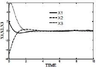
Fig.2 Evolution of state variables with time

Fig.3 Evolution of sliding surface

(6)

SUPER TWISTING CONTROLLER

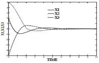
Fig.6 Evolution of state variables with time

IV.POLE ASSIGNMENT FOR SLIDING MODE CONTROL

We consider the linear-time invariant system Ẋ=Ax+Bu

Y=Cx+Du

We look for a state gain K such that U=-Kx

In this case we have the closed loop system

̇

= Ax-BKx =(A-BK)x

We should note that we can modify the dynamics of the system by state feedback. If the system is controllable, it is always possible to find a state gain K to set the Eigen values of the closed loop system at arbitrary values.

(7)

1. Quadratic optimal control 2. Mayne-Murdoch formula 3. Ackerman’s formula 4. Bass-Gura formula

EXAMPLE: INVERTED PENDULUM

QUADRATIC OPTIMAL CONTROL

Table.2 Gain values

Fig.8 Convergence of state variables

MAYNE-MURDOCH FORMULA

(8)

ACKERMAN’S FORMULA

Table.4 Gain values

BASS-GURA FORMULA

(9)

APPLYING THE VALUES OF K TO THE SLIDING MODE CONTROL

Converting the matrix into the regular form we get

CONSTANT RATE REACHING LAW

Fig.12 EVOLUTION OF STATE VARIABLES

CONSTANT PLUS PROPORTINAL RATE REACHING LAW

(10)

SUPER TWISTING CONTROLLER

Fig.14 EVOLUTION OF STATE VARIABLES

V. CONCLUSION

Sliding mode control is used to study the robust behavior of the system even in the presence of the uncertainties. The behavior of chemical systems is studied so that the state variables converge asymptotically to the equilibrium. The control law is designed in such a way that the state variables slide along the sliding surface and reach the equilibrium asymptotically. The continuous and discontinuous control modes were studied and the results are obtained. The sliding mode control produces the desired performance even in the presence of uncertainty. The poles are assigned to the systems to obtain the desired performance using few methods. Tracking is also incorporated to the systems.

REFERENCES

[1] Nishat Anwar Md , Shamsuzzoha M , Somnath Pan. A frequency domain PID controller design method using direct synthesis approach. Arab JsciEng. 2015;40:995-1004.

[2] Vijayan V , Rames C.Panda. Design of PID controllers in double feedback loops for SISO system with set point filters. ISA Transactions 51. 2012;514-521.

[3]Sivaramakrishnan S, Tangirala A.K , Chidambaram M. Sliding Mode For Unstable System.Chem.BioChem,Eng.Q.22(1).2008;41-47.

[4] John Y. Hung, Member, IEEE,Weibing Gao,Senior Member,IEEE, and James C.Hung, Fellow, IEEE. IEEE transactions on industrial electronics, Vol.40,No