Time Series Seasonal Analysis Based on Fuzzy Transforms

Type of the Paper (Article)

1

Time Series Seasonal Analysis Based on Fuzzy Transforms

2

3

Ferdinando Di Martino1,* _{and Salvatore Sessa}1

4

1 _{Università degli Studi di Napoli Federico II, Dipartimento di Architettura, via Toledo 402, 80134 Napoli}

5

(Italy); fdimarti,[email protected]

6

* Correspondence: [email protected]; Tel.: +39-081-253-8907; Fax: +39-081-253-8905

7

8

Abstract: We define a new seasonal forecasting method based on fuzzy transforms. We use the best

9

interpolating polynomial for extracting the trend of the time series and generate the inverse fuzzy

10

transform on each seasonal subset of the universe of discourse for predicting the value of a an

11

assigned output. Like first example, we use the daily weather dataset of the municipality of Naples

12

(Italy) starting from data collected from 2003 till to 2015 making predictions on the following

13

outputs: mean temperature, max temperature and min temperature, all considered daily. Like

14

second example, we use the daily mean temperature measured at the weather station “Chiavari

15

Caperana” in the Liguria Italian Region. We compare the results with our method, the average

16

seasonal variation, ARIMA and the usual fuzzy transforms concluding that the best results are

17

obtained under our approach in both examples.

18

19

Keywords: ARIMA; forecasting; fuzzy partition; fuzzy transform; time series

20

21

1. Introduction

22

Time series forecasting methods are quantitative techniques that analyse historical data of a

23

variable for predicting its values. Traditional forecasting methods [1, 2, 3, 4, 14, 19, 20] use statistical

24

techniques to estimate the future trend of a variable starting from numerical datasets. Many time

25

series data contain seasonal patterns, that is regular, repetitive and predictable changes that happen

26

sequentially in a period of time which could be a year, a season, a month, a week, etc.

27

Different approaches have been developed to deal with trend and seasonal time series.

28

Traditional approaches, such the moving average method, additive and multiplicative models,

29

Holt-Winters exponential smoothing, etc. [3, 4, 14, 20], use statistical methods for removing the

30

seasonal components: they decompose the series into trend, seasonal, cyclical and irregular

31

components [32]. Other statistical approaches are based on the Box–Jenkins model, called

32

Autoregressive Integrated Moving Average (ARIMA) [3, 14, 20, 25]. In the first phase of the

33

model ARIMA an auto-correlation analysis is performed for verifying if the series is non-stationary,

34

then the series is transformed into a stationary series formed by the differences between the value at

35

the actual moment and the value at the previous moment.

36

The main limitation of the seasonal ARIMA model is the fact that the process is considered to be

37

linear. Many soft computing models have been presented in literature for capturing nonlinear

38

characteristics in seasonal time series like, e. g., Support Vector Machine ( SVM) [21, 24] used for

39

wind speed prediction [22], air quality forecasting [18], rainfall forecasting [13]. SVM utilizes a

40

kernel function to transform the input variables into a multi-dimensional feature space, then the

41

Lagrange multipliers are used for finding the best hyperplane to model the data in the feature space.

42

The main advantage of an SVM method is that that the solution is unique and there are no risk to

43

move towards local minima, but some problems remain as the choice of the kernel parameters which

44

influences the structure of the feature space, affecting the final solution. Another method is based on

45

an Artificial Neural Network (ANN) [5, 12, 32, 31]. The most widely used ANN architectures for

46

forecasting problems are given by multi-layer Feed Forward Network (FNN) architectures [29, 30],

47

where the input nodes are given by the successive observations of the time series, that is the target yt

48

is a function of the values yt-1, yt-2,…, yt-p , where p is the number of input nodes.

49

A variation of FNN is the Time Lagged Neural Network (TLNN) architecture [9,16], where the

50

input nodes are the time series values at some particular lags. For example, in a time series having

51

the month as seasonal period, the neural network used for forecasting the parameter value at the

52

time t can contain input nodes corresponding to the lagged values at the time t-1, t-2,..,t-12. The key

53

point is that an ANN can be considered a nonlinear auto-regression model. ANN’s are inherently

54

nonlinear and can model accurately complex characteristics in data patterns with respect to linear

55

approaches such as ARIMA models. One of the main problems in the ANN forecasting models is the

56

selection of appropriate network parameters. This operation is crucial since it affects strongly the

57

final results. Furthermore, the presence of a high number of network parameters in the model can

58

produce overtraining of data, giving rise to incorrect forecasting solutions.

59

In order to reduce the problems present in the SVM and ANN approaches, some authors have

60

recently developed some hybrid models like, e.g., genetic algorithms and tabu search (GA/TS) [24]

61

and the Modified Firefly Algorithm (MFA).

62

In [15] a Discrete Wavelet Transform (DWT) algorithm is used to decompose the time series into

63

linear and nonlinear components, afterward the ARIMA and the ANN models are used to

64

forecasting separately the two components.

65

In [27] the authors present four seasonal forecasting models: an adaptive ANN model that uses

66

a genetic algorithm for evolving the ANN topology and the back-propagation parameter, a SVM

67

seasonal forecasting model and two hybrid ANN and SVN models based on linguistic fuzzy rules.

68

The authors compare the four methods with the traditional ARIMA method, showing that the

69

results under the four methods are comparable with the ones obtained using ARIMA. The best

70

results are obtained by using the adaptive ANN algorithm based on linguistic fuzzy rules but

71

ANN-based methods are complex to manage and require more computational effort.

72

In order to overcome this high computational complexity and the heavy dependence on the

73

input parameters, a soft computing forecasting method based on fuzzy transforms [26] (for short,

74

F-transforms) is presented in [6]. There this method was applied to the North Atlantic Oscillation

75

(NAO) data time series; the results are better than the ones obtained by using the well known

76

Wang-Mendel method [28] and Local Linear Wavelet Neural Network ( LLWNN) techniques.

77

The F-transforms are a powerful flexible method to be applied in various domains such as

78

image compression [8], detection of attribute dependencies in data analysis [7] and extraction of the

79

trend cycle of time series [23].

80

Strictly speaking, in [6] a forecasting index is calculated with respect to the data of the training

81

set: if this index is smaller than or equal to an assigned threshold, the algorithm is stopped,

82

otherwise it is iterated by taking a finer fuzzy partition of the variable domain. When a fuzzy

83

partition is settled, the algorithm controls that the training dataset is sufficiently dense with respect

84

to the fuzzy partition, that is each fuzzy set of the fuzzy partition has at least a non-zero membership

85

degree in some point.

86

Here we give a forecasting method based on F-transforms for seasonal time series analysis

87

called Time Series Seasonal F-transform (TSSF). We give a partition of the time series dataset into

88

seasonal pattern components. A seasonal pattern is related to a fixed period of the time series

89

fluctuations: the seasonality is set on a fixed period such as year, month, week, etc. In the TSSF

90

model we assume that the different components affect the time series. We use the best polynomial fit

91

for estimating the trend of the time series. After de-trending the data by subtracting the trend from

92

the time series dataset, we find a fuzzy partition of the dataset into seasonal subsets to which we

93

apply the F-transforms by checking that the chosen partition is optimal for the density of the training

94

data. In [6, 7] the authors have developed this process: in particular, four forecasting indexes are

95

proposed for assessing the quality of the results: Mean Absolute Deviation (MAD), Mean Absolute

96

Percentage Error (MAPE), Root Mean Square Error (RMSE) and Mean Absolute Deviation Mean

(MADMEAN). An optimal fuzzy partition is found by calculating the corresponding RMSE and

98

MADMEAN: if at least one of the two indices does not exceed a respective threshold, then the

99

process stops and the given fuzzy partition is considered optimal.

100

In the TSSF method we essentially adopt the same procedure but we prefer to use the

101

MADMEAN index because that this index is more robust than other forecasting indexes, as proved

102

in [17]. We emphasize that the dimension of the optimal fuzzy partition can vary with the seasonal

103

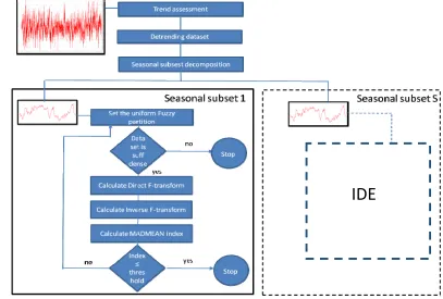
subset. In Fig. 1 the TSSF method is synthetized in detail.

104

In the assessment phase the best polynomial fit is applied for determining the trend in the

105

training data. After de-trending the dataset, the time series is decomposed into S seasonal subsets to

106

which the F-transform forecasting iterative method is applied. Initially, a coarse grained uniform

107

fuzzy partition is fixed. If the subset is not sufficiently dense with respect to the fuzzy partition, the

108

F-transform sub-process applied on the seasonal subset stops, else the MADMEAN index is

109

calculated and if it is greater than an assigned threshold, the F-transform sub-process is iterated

110

considering a finer uniform fuzzy partition. The output is given by the inverse F-transforms

111

obtained for each seasonal subset at the end of the corresponding sub-process.

112

113

Figure 1. Schema of the TSSF method.

114

115

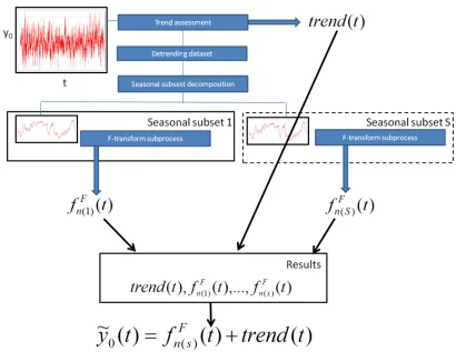
To forecast a value of a parameter y0 at the time t we calculate the sth seasonal subset of

116

cardinality n(s) in which the time t is inserted. Then we consider the sth inverse F-transform

117

)

(

)

(

t

f

F s

n . The forecasted value of the parameter is given by the formula

118

)

(

)

(

)

(

t

trend

t

f

F

s

n

+

,

119

where trend(t) is the value of the polynomial trend at the time t. Fig. 2 illustrates the application of

120

the TSSF for forecasting analysis.

121

122

123

124

Figure 2. The TSSF method for forecasting analysis.

125

126

For sake of completeness, we recall the concept of F-transform in Section 2. Section 3 contains

127

the F-transform-based prediction method, in Section 4 we describe our TSSF method applied on the

128

climate dataset of the municipality of Naples (www.ilmeteo.it/portale/archivio-meteo/Napoli)

129

whose results are given in Section 5 that containin also comparisons with average seasonal variation,

130

ARIMA and traditional prediction F-transform methods. Section 6 reports the final conclusions.

131

132

2. Direct and inverse f-transform

133

Following the definitions and notations of [26], let n ≥ 2 and x1, x2, …, xn be points of [a,b],

134

called nodes, such that x1 = a < x2 <…< xn = b. The family of fuzzy sets A1,…,An : [a,b] → [0,1], called

135

basic functions, is a fuzzy partition of [a,b] if the following hold:

136

137

- Ai(xi) =1 for every i =1,2,…,n;

138

- Ai(x) = 0 if x

∈

]xi-1,xi+1[ for i = 2,…,n-1;

139

- Ai(x) is a continuous function on [a,b];

140

- Ai(x) strictly increases on [xi-1, xi] for i = 2,…, n and strictly decreases on [xi,xi+1]

141

for i = 1,…, n-1;

142

- A1(x) +…+ An(x) = 1 for every x

∈

[a,b].

143

144

The fuzzy sets {A1(x),…,An(x)} form an uniform fuzzy partition if

145

146

- n ≥ 3 and xi = a + h∙(i-1), where h = (b-a)/(n-1) and i = 1, 2, …, n (that is the nodes are

147

equidistant);

148

- Ai(xi – x) = Ai(xi + x) for every x

∈

[0,h] and i = 2,…, n-1;

149

- Ai+1(x) = Ai(x - h) for every x

∈

[xi, xi+1] and i = 1,2,…, n-1.

Here we only interested in the discrete case, that is to functions f defined on the set P of points

151

p1,...,pm of [a,b]. If P is sufficiently dense with respect to the fixed partition{A1, A2, …, An}, that is for

152

each i

∈

{1,…,n} there exists an index j

∈

{1,…,m} such that Ai(pj) > 0, we can define the n-tuple {F1, F2,

153

…, Fn } as the discrete direct F-transform of f with respect to the basic functions {A1, A2, …, An },

154

where Fi is given by

155





= =

=

_m

j i j

m j j i j

p

A

p

A

p

f

F

1 1 i

)

(

)

(

)

(

(1)

for i=1,…,n. Similarly we define the discrete inverse F-transform of f with respect to the basic

156

functions {A1, A2, …, An} by setting

157

)

(

)

(

1 j i n i i j F

n

p

F

A

p

f



=

=

(2)

for every j

∈

{1,…,m}. We can extend the above concepts to functions in k (≥2) variables. In the

158

discrete case, we assume that the function f(x1,x2,…, xk) is defined on m points pj = (pj1, pj2,…,pjk)

∈

159

[a1,b1]×[a2,b2]×…×[ak,bk] for j=1,…,m. We say that P={(p11, p12, …, p1k), …, (pm1, pm2, …,pmk)} is

160

sufficiently dense with respect to the fuzzy partitions

161

{

A

11

,

A

12

,...,

A

1n1

}

,...,

{

A

k1

,

A

k2

,...,

A

knk

}

(3)

of [a1,b1],…, [ak,bk], respectively, if for each k-tuple {h1,…,hk}

∈

{1,…,n1}×…×{1,…,nk}, there exists

162

a point pj = (pj1, pj2,…,pjk) in P, j=1,…,m, such that ₁

(

₁

)

...

(

)

0

.

1 j

⋅

⋅

kh jk

>

h

p

A

p

A

k

163

In this case we define the (h1,h2,…,hk)-th component

k h h h

F

_... 2

1 of the discrete direct

164

F-transform of f with respect to the basic functions as

165

 = ⋅ ⋅ ⋅  = ⋅ ⋅ ⋅ ⋅ = _m j jk p k kh A j p h A j p h A m j jk p k kh A j p h A j p h A jk p j p j p f k h h h F 1 ) ( ... ) 2 ( 2 2 ) 1 ( 1 1 1 ) ( ... ) 2 ( 2 2 ) 1 ( 1 1 ) ,... 2 , 1 ( ... 2 1 (4)

Now we define thediscrete inverse F-transform of f with respect to the above basic functions

166

to be the following function by setting for each point pj =(pj1, pj2,…,pjk)

∈

[a1,b1]× …× [ak,bk]:

167

(

)

( )

j kh

( )

jk

n

h n

h n

h hh h h

jk j

F n

n

p

p

F

A

p

A

p

f

k k

k

k

k

,....,

...

1

...

1 1 1 ... 11

1 ... 1 1 2 2 2 1

1

  

= = =

⋅

=

(5)

for j=1,…,m. The following theorem holds [26]:

168

169

Theorem. Let f(x1,x2,…,xk) be given on the set of points P = {(p11,p12, …,p1k) ,(p21, p22, …, p2k),

170

…,(pm1, pm2, …,pmk)}

∈

[a1,b1]×[a2,b2]× …×[ak,bk]. Then for every ε > 0, there exist k integers

171

n1=n1(ε),…,nk=nk(ε) and k related fuzzy partitions (3) of [a1,b1], …, [ak,bk], respectively, such that the

172

set P is sufficiently dense with respect to them and for every pj = (pj1, pj2,…,pjk) in P, j=1,…,m, the

173

following inequality holds:

174

(

)

−

_k

(

j jk

)

<

ε

F

n n jk

j

p

f

p

p

p

f

1

,...,

1... 1

,...,

(6)

We now describe the F-transform forecasting algorithm presented in [6]. Let M be assigned

176

input-output pairs data (x(j)_{, y}(j)_{) in the following form:}

177

) y , ,..., , ... , ( ) y , ( ... ) y , ..., ,..., ( ) y , ( ... ) y , ..., ..., , ( ) y , ( (M) ) ( ) ( ) ( (M) ) ( (j) ) ( ) ( ) ( (j) ) ( (1) ) 1 ( ) 1 ( ) 1 ( (1) ) 1 ( 1 1 1 M n M M M j n j i j j n i x x x x x x x x x i = = = x x x (7)

for j = 1,2, …,M. The task is to generate a fuzzy rule-set from the M pairs (x(j)_{, y}(j) _{) in order to}

178

determine a mapping f from the input-space Rn _{into the output-space R. We assume that the}

179

) ( ) ( ) 1

( _{,..., ,...,} M i j i

i x x

x lie in

[

−, +

]

i i x

x for every i=1,…,n, and y(1)_{, y}(2)_{,…, y}(M) _in[y−_,y+_{]. The F-transform}

180

forecasting method calculates a function

y

=

f

(

x

₁

,...,

x

_n

)

which approximates the data. Like in [7],

181

we create a partition of ni fuzzy sets for each domain

[

x

_i−

,

x

_i*

]

, hence we construct the respective

182

direct and the inverse F-transforms (3) and (4) in order to estimate an approximation of f. We

183

illustrate this forecasting method in the following steps:

184

1) give an uniform partition composed by ni fuzzy sets (ni ≥3)

{

A

_i1

,...,

A

_ini

}

of the domain

185

]

,

[

* i i

x

x

− _{of each variable xi, i = 1,…,n. If}

i

in is

i

x

x

x

₁

,...,

,...,

are the nodes of each

186

interval

[

x

_i−

,

x

*_i

]

, each function Ais is defined in the following way for s=1,…,ni:

187

otherwise 0 ] , [ x if )) ( cos 1 ( 5 . 0 ) ( otherwise 0 ] x , [x x if )) ( cos 1 ( 5 . 0 ) ( otherwise 0 ] x , [x x if )) ( cos 1 ( 5 . 0 ) ( ) 1 ( ) 1 ( 1) i(s 1) -i(s i2 i1 1 1     _{⋅ + − ∈} =     _{⋅ + − ∈} =     _{⋅ + − ∈} = − − + i i i i in n i n i i in is i is i i i x x x x s x A x x s x A x x s x A π π π (8)

where

x

i1

=

x

i−,

x

ini

=

x

i+,

=

(

−

)

/

(

−

1

)

− +

i i i

i

x

x

n

s

and

x

_is

=

x

_i−

+

s

_i

⋅

(

s

−

1

)

;

188

2) if the dataset is not sufficiently dense with respect to the fuzzy partition, that is if

189

there exists a variable xi and a fuzzy set Ais of the corresponding fuzzy partition such

190

that ( (r))₌0

i is x

A for each r = 1,…,M, the process stops otherwise calculate the

191

n1∙n2∙…∙nk components of the direct F-transform of f with (3) by setting k=n,

192

) ( 1 1 j j

x

p

=

,…,p_jn=x_n(j) and y(j)= f(x₁(j),x(₂j),...,x_n(j)), obtaining the following:

193





= =

⋅

⋅

⋅

⋅

⋅

=

M j j n h n j h M j j n nh j h j h h h

x

A

x

A

x

A

x

A

y

F

n n n 1 ) ( ) ( 1 1 1 ) ( ) ( 1 1 ) ( ...

)

(

...

)

(

)

(

...

)

(

1 1 2 1 (9)

3) calculate the discrete inverse F-transform as

194

(

)

 

= = =

⋅

⋅

⋅

=

1 1 2 2 1 1 2 1 1 1

1 1 1

) ( ) ( 1 ... ) ( ) ( ...

,....,

...

(

)

...

(

)

n h n h n h j n nh j h h h h j n j F n n n n n n

n

x

x

F

A

x

A

x

f

(10)

to approximate the function f;

196

4) calculate the forecasting index as

197





= =

−

=

M j j M j j j n j F n n n

y

y

x

x

f

MADMEAN

n 1 ) ( 1 ) ( ) ( ) ( 1 ...

(

,...,

)

2 1 (11)

If it is less or equal to an assigned threshold, then the process stops otherwise a finer fuzzy

198

partition is taken and the process restarts from the step 2.

199

In [6] four forecasting indices RMSE, MAPE, MAD, MADMEAN were proposed, but we

200

prefer to use MADMEAN which is the best one in terms of accuracy as proved in [17].

201

4. TSSF method

202

We consider time series of data formed from observations of a original parameter y0 measured

203

at different times. The dataset is formed by M measure pairs as

(

t

(0)

,

y

₀(0)

) (

,

t

(1)

,

y

₀(1)

) (

,...,

t

(M)

,

y

₀(M)

)

.

204

Our aim is to evaluate seasonal fluctuations of a time series by using the F-transform method.

205

First of all, we use a polynomial fitting for calculating the trend of the phenomenon with respect to

206

the time. Afterwards we subtract the trend from the data obtaining a new dataset of the fluctuations

207

y(j) _being ( )

(

( )

)

0 )

(j

_y

j

_trend

_t

j

y

=

−

. After de-trending the dataset, it is partitioned into S subsets,

208

being S seen as seasonal period. Each subset represents the seasonal fluctuations with respect to the

209

trend.

210

The seasonal data subset is composed by Ms pairs, expressing the fluctuation measures of the

211

parameter y0 at different times: (t(1) _{, y}(1)_{), (t}(2) _{, y}(2)_{).... (t(Ms) , y(Ms)), where y}(i) _{is given by the original}

212

measure

y

₀(j)at the time t(j) _{minus the trend calculated at this time. The formulae of the}

213

corresponding one-dimensional directed and inverse F-transforms, considering n basic functions,

214

are given as

215





= =

⋅

=

S S M j j h M j j h j h

t

A

t

A

y

F

1 ) ( 1 ) ( ) (

)

(

)

(

(12)



=

⋅

=

n

h h h

F

n

t

F

A

t

f

1

)

(

)

(

(13)

respectively. The inverse F-transform (13) approximates the seasonal fluctuation at the time t. In our

216

method we start with three basic functions and verify that the subset of data is sufficiently dense

217

with respect to this fuzzy partition. After calculating the directed and inverse F-transform using (12)

218

and (13), respectively, we calculate the (MADMEAN)s index for the sth fluctuation subset of data

219

given as

220





= =

−

=

_s s M j j M j j j F n s

y

y

t

f

MADMEAN

1 ) ( 1 ) ( ) (

₎

(

)

(

(14)

If the MADMEAN index (14) is greater than an assigned threshold, than the process is iterated

221

considering a fuzzy partition of dimension n:= n+1, otherwise the iteration process stops. Our

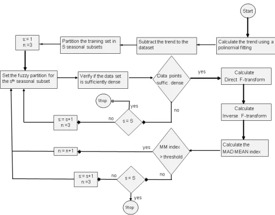
222

algorithm is illustrated in Fig. 3.

225

Figure 3. Flux diagram related of the TSSF method.

226

227

For the sth fluctuation subset, we obtain the inverse F-transform by using the following n(s)

228

basic functions:

229



=

⋅

⋅

=

( )

1 )

(

(

)

(

)

s

n

h

h h F

s

n

t

F

A

t

f

(15)

For evaluating the value of the parameter y0 at the time t in the sth seasonal period, we add to

230

)

(

) (

t

f

F s

n the trend calculated at the time t obtaining the following value:

231

)

(

)

(

)

(

~

) (

0

t

f

t

trend

t

y

F

s

n

+

=

(16)

For evaluating the accuracy of the results, we can use the MADMEAN index, given by:

232





=

= −

= M

j j M

j

j j

y y t y MADMEAN

1 ) ( 0 1

) ( 0 ) (

0( )

~

(17)

For sake of completeness, we describe also the values of the above cited indices:

233

- the Root Mean Square Error (RMSE) defined as

234

(

)

1/2

1

2 ) ( 0 ) (

0

(

)

~





















₋

=



=

M

y

t

y

RMSE

M

j

j j

(18)

- the Mean Absolute Percent Error (MAPE) defined as

235



=

−

=

M

j j

j j

y

y

t

y

M

MAPE

1 ₀( )

) ( 0 ) (

0

(

)

~

1

(19)

- the Mean Absolute Deviation (MAD), defined as

M

y

t

y

MAD

M

j

j j



=

−

=

1

) ( 0 ) (

0

(

)

~

(20)

To evaluate the MADMEAN threshold we apply the k-cross-validation technique in order to

237

control the presence of overfitting in the learning data. We set a seasonal subset and partition it

238

randomly in k folds. The union of k-1 folds is used as a training set and the other fold is used as a

239

validation set. Then we consider a fuzzy partition size n = 3 and apply the TSSF algorithm to the

240

training set calculating the MADMEAN index; then we use the validation test to calculate the RMSE

241

index. We repeat this process for the k combination of k-1 folds used as a training test and a fold

242

used as validation set. Then, we obtain the mean MADMEAN and RMSE indexes as:

243

k

n MADMEAN n

MADMEAN

k

i

i



= = 1

) ( )

( (21)

k n RMSE n

RMSE

k

i

i



= = 1

) ( )

( (22)

where MADMEAN(n) and RMSE(n) are the mean MADMEAN and RMSE by using the fuzzy

244

partition size n.

245

We repeat this process by using many values of n; then we plot in a graph the RMSE(n) by

246

varying the fuzzy partition size n. The threshold value is set as the mean MADMEAN value

247

obtained in correspondence of the fuzzy partition size n in which there is a plateau in the RMSE

248

graph. In our tests we set k = 10.

249

5. Experiments on time series data

250

We compare the results obtained by using the TSSF method with the one obtained by using

251

three other seasonal forecasting methods: a simple average variation method, the seasonal ARIMA

252

and the F-transforms prediction method. The training dataset is composed from climate data (mean,

253

maximum and minimum temperature, pressure, speed of the wind, etc., measured every day ) of the

254

municipality of Naples collected at web pages: www.ilmeteo.it/portale/archivio-meteo/Napoli. The

255

main climate parameters are measured every thirty minutes and are the following: Min temperature

256

(°C), Mean temperature (°C), Max temperature (°C), Dew point (°C), Mean humidity (% ), Mean

257

view (km), Mean wind speed (km/h), Max wind speed (km/h), Gust of wind (km/h), Mean pressure

258

on sea level (mb), Mean pressure (mb), Millimetres of rain (mm).

259

For sake of brevity, we limit the results for the parameters mean, max and min temperature. As

260

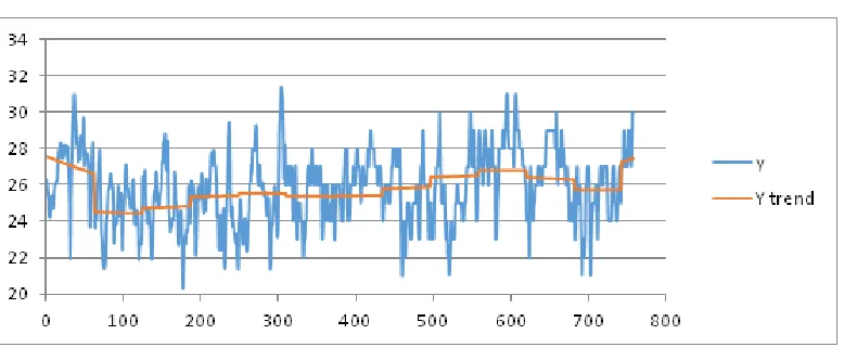
training dataset, we consider these data recorded in the months July and August from 01/07/2003

261

to 16/08/2015, hence for overall 806 days represented as abscissas (via a number ID) in Fig.s 4 and 6,

262

respectively. The daily mean and max temperature is represented on the ordinate axis in Fig.s 4 and

263

6, respectively. We obtain the best fit polynomial of nine degree ( i

i i

x

a

y

=



⋅

=

9

1

) (red color in Fig.s 4

264

and 6) whose coefficients are given in Appendix.

267

Figure 4. Trend of the mean temperature in the months of July and August (from 01/07/2003 till to

268

16/08/2015) obtained by using a ninth-degree polynomial fitting.

269

We consider the week as seasonal period, partitioning the data set into 9 seasonal subsets: week

270

27 (01/07) to the week 36 (31/08). We apply the TSSF method by setting the threshold of the

271

MADMEAN index to 6%. For the daily mean and max temperature, we have also used the below

272

other three methods, whose the final results have been plotted in Fig.s 5a÷5d and Fig.s 7a÷7d,

273

respectively.

274

1) Average seasonal variation method (labelled as avgSV). This method calculates the mean

275

seasonal variation for each seasonal period and adds the mean seasonal variation to the trend value.

276

2) Seasonal ARIMA method. In our experiments we used the forecasting tool ForecastPro [11].

277

As highlighted in [27], this tool is is well known by ensuring the best performance in the use of

278

forecasting ARIMA models.

279

3) F-transform prediction method [6] applied to the complete dataset (labelled as F-transforms).

280

281

282

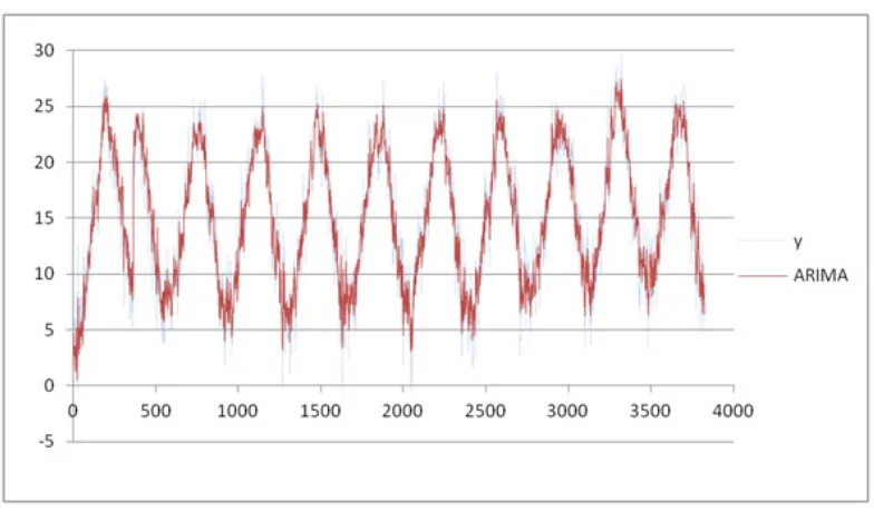
Figure 5a. Results obtained for the mean temperature by using the avgSV method.

283

Figure 5b. Results obtained for the mean temperature by using the ARIMA method.

285

286

Figure 5c. Results obtained for the mean temperature by using the F-transforms method.

287

288

289

Figure 5d. Results obtained for the mean temperature by using the TSSF method.

290

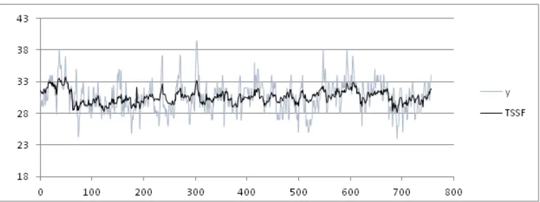
In Table 1 we show the four indices obtained by using the four methods. The best results for the

291

mean temperature are obtained using the TSSF method whose MADMEAN is 4.22%.

292

Table 1. RMSE, MAPE, MAD and MADMEAN indices for the mean temperature

293

Forecasting

method RMSE MAPE MAD MADMEAN

avgSV 1.78 5.60% 1.42 5.50%

ARIMA 1.55 4.89% 1.24 4.80%

F-transforms 1.61 4.96% 1.28 5.05%

TSSF 1.37 4.29% 1.09 4.22%

294

295

Figure 6. Trend of the max temperature in the months of July and August (from 01/07/2003 till to

296

298

Figure 7a. Results for the max temperature in the months of July and August under avgSV method.

299

300

Figure 7b. Results for the max temperature in the months of July and August under Arima method.

301

302

Figure 7c. Results for the max temperature in the months of July and August under the F-transforms

303

method.

304

305

Figure 7d. Results for the max temperature in the months of July and August under the TSSF

306

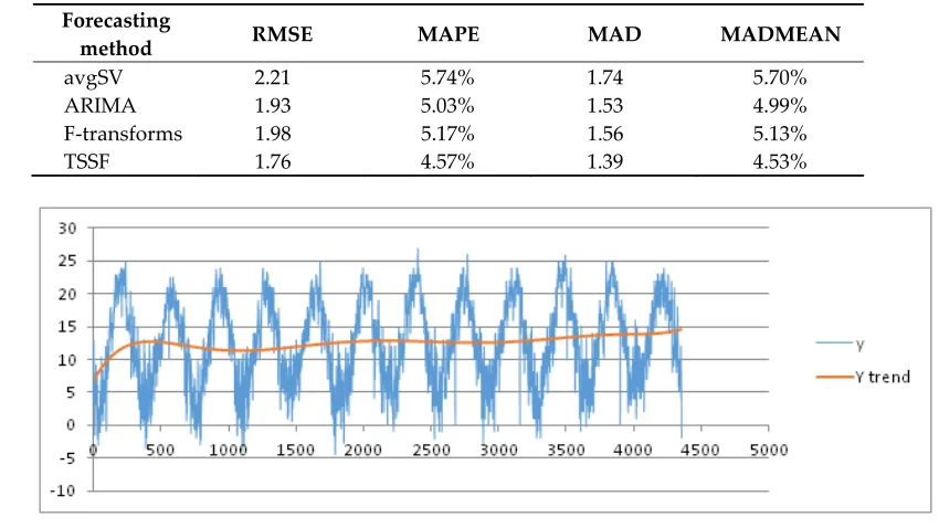
In Table 2 we show the four indexes obtained by using the four methods. The best results for the

308

max temperature are obtained by using TSSF whose MADMEAN index is 4.56%.

309

Now we present the results of other experiments in which the variation of the min temperature

310

is explored during the years. Now we assume a month as seasonal period: the training dataset is

311

formed by all the measures recorded from 01/01/2003 to 31/12/2015. It is partitioned into 12 seasonal

312

subsets corresponding to the 12 months of a year. In Fig. 8 we show the data and the trend obtained

313

by using a best fit polynomial of nine degree (see Appendix).

314

Table 2. RMSE, MAPE, MAD and MADMEAN indices for the max temperature

315

Forecasting

method RMSE MAPE MAD MADMEAN

avgSV 2.21 5.74% 1.74 5.70%

ARIMA 1.93 5.03% 1.53 4.99%

F-transforms 1.98 5.17% 1.56 5.13%

TSSF 1.76 4.57% 1.39 4.53%

316

317

Figure 8. Trend of min temperature under a best fit polynomial of nine degree.

318

319

Figure 9a. Results obtained for the variation of the min temperature by using the avgSV method.

320

Figure 9b. Results obtained for the variation of the min temperature by using the ARIMA method.

322

323

324

Figure 9c. Results obtained for the variation of the min temperature by using the F-transforms

325

method.

326

327

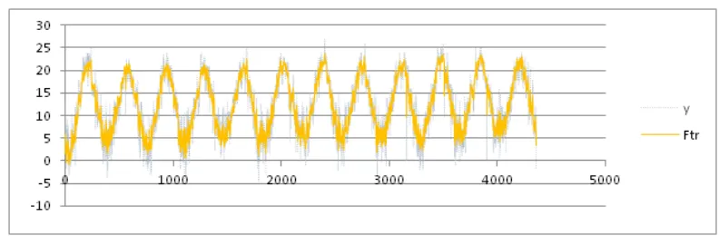
Figure 9d. Results obtained for the variation of the min temperature by using the TSSF method.

328

As we can observe in Fig.8, the seasonality of the data seems more evident than in the two

329

previous examples. In Fig. 9a÷9d we have plotted the final results by using the four forecasting

330

methods.

331

In Table 3 we show the indices obtained by using the four methods, the MAPE index is not

332

measurable because there are measures of min temperature equal to 0. As for the results obtained

333

previously, the best results for the min temperature are obtained by using the TSSF, whose

334

MADMEAN is 5.26%.

335

Table 3. RMSE, MAPE, MAD and MADMEAN indices for the min temperature

336

Forecasting

method RMSE MAPE MAD MADMEAN

avgSV 2.97 - 2.34 18.66%

ARIMA 1.25 0.97 7.46%

F-transforms 1.56 - 1.09 8.73%

TSSF 0.87 - 0.66 5.26%

337

The results in Table 3 show that the TSSF is more efficient when the seasonality of the data is

338

more pronounced as for the mean temperature time series. In order to test the reliability of the

339

forecasting results obtained by using the four forecasting methods, we have considered test datasets

340

containing the measure of the analysed parameter in a next time period and calculating the RMSE

341

obtained with respect to the forecasted values. For the mean and max temperature parameters we

342

use a test dataset formed by the mean and max daily temperatures measured in the interval

343

17/08/2015 – 31/08/2015. For the min temperature parameter we use a test dataset formed by the min

daily temperatures measured in the interval 01/01/2015-31/08/2015. In Table 4 we show the RMSE

345

measured in the four methods for each of the three parameters.

346

347

Table 4. RMSE measured in the four methods

348

Parameter

Training dataset dimension

Test dataset dimension

Seasonal

period RMSE

avgSV ARIMA F-transf. TSSF

Temp. mean 757 15 Week 1.83 1.58 1.62 1.39

Temp. max 757 15 Week 2.20 1.92 1.99 1.68

Temp. min 4354 212 Month 2.90 1.27 1.54 0.94

349

These results confirm that the best performances are obtained by using the TSSF algorithm: the

350

most reliable results are obtained for the third parameter in which the seasonality is more regular.

351

We repeated these comparison tests by using other climatic datasets. For brevity we show the

352

results obtained analysing the trend of the daily mean temperature measured at the weather station

353

Chiavari Caperana in the Liguria Italian Region; the data can be downloaded at the web site

354

http://www.cartografiarl.regione.liguria.it/SiraQualMeteo/script/PubAccessoDatiMeteo.asp of the

355

Liguria Region web page “Ambiente in Liguria”.

356

The analyzed data concern the measures in °C of the daily mean temperature in the period

357

01/01/2006 - 31/12/2016. The month is set as the seasonal period; the dataset it is partitioned into 12

358

seasonal subsets corresponding to the 12 months of a year.

359

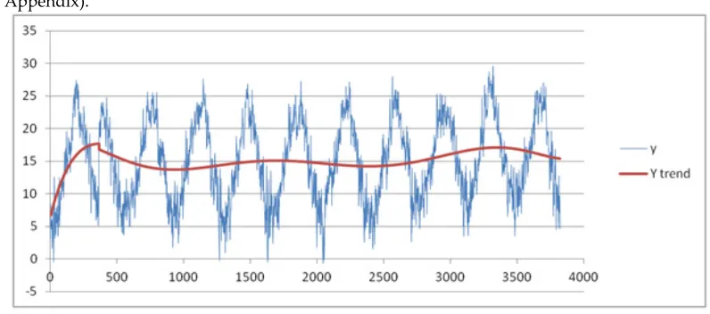
In Fig. 10 we show the data and the trend obtained by using a best fit polynomial of nine degree

360

(see Appendix).

361

362

Figure 10. Trend of mean temperature under a best fit polynomial of nine degree - Chiavari

363

365

Figure 11a. Results obtained for the variation of the min temperature by using the avgSV method.

366

367

369

Figure 11c. Results obtained for the variation of the min temperature by using the F-transforms

370

method.

371

372

Figure 11d. Results obtained for the variation of the min temperature by using the TSSF method.

373

In Table 5 we show the four indexes obtained by using the four methods. The best results for the

374

mean temperature are obtained by using TSSF whose MADMEAN index is 3.83%.

375

Table 5. RMSE, MAPE, MAD and MADMEAN indices for the mean temperature (Chiavari

376

Caperana weather station)

377

Forecasting

method RMSE MAPE MAD MADMEAN

avgSV 2.87 27.74% 2,14 16.19%

ARIMA 1.13 12.37% 0.89 5.95%

F-transforms 1.38 15.18% 1.10 7.30%

TSSF 0.73 7.96% 0.58 3.83%

378

The results in Table 5 confirm the ones obtained for the min temperature parameters in the

379

weather dataset of the Municipality of Naples in Table 3: the TSSF gives better results than the

380

ARIMA and F-transform algorithms and is more efficient when the seasonality of the data is more

381

pronounced. In order to test the reliability of the results obtained in Table 5, we have considered a

382

test dataset containing the measure of the daily mean temperature in the period

01/01/2017-19/03/2017 and calculating the RMSE obtained with respect to the forecasted values. In

384

Table 6 we show the RMSE measured in the four methods for each of the three parameters.

385

386

Table 6. RMSE measured in the four methods for the mean temperature (Chiavari Caperana weather

387

station)

388

Parameter

Training dataset dimension

Test dataset dimension

Seasonal

period RMSE

avgSV ARIMA F-transf. TSSF

Temp. mean 3822 78 Month 2.85 1.15 1.40 0.81

Temp. max 757 15 Week 2.20 1.92 1.99 1.68

Temp. min 4354 212 Month 2.90 1.27 1.54 0.94

389

Also the results in Table 6 confirm that the best performances are obtained by using the TSSF

390

algorithm. In the other tests we obtain the same results; the results show that the better

391

performances are obtained by using the TSSF algorithm and the most reliable results are obtained

392

when the seasonality is more regular.

393

In Table 7 we show the tests results obtained for the mean temperature by using the seasonal

394

datasets of the daily mean temperature measured by other stations in the district of Genova; the data

395

were downloaded from the Liguria Region web page “Ambiente in Liguria”. In each experiment the

396

season parameter is given by the month of the year.

397

398

Table 7.RMSE measured in the four methods for the mean temperature in different station in the district

399

of Genova (Italy):

400

Station RMSE

avgSV ARIMA F-transf. TSSF

Alpe Gorreto 2.98 1.20 1.49 0.84

Campo Ligure 2.74 1.09 1.34 0.76

Barbagelata 3.25 1.30 1.57 0.89

Camogli 3.39 1.38 1.68 0.95

Campo ligure 3.02 1.20 1.49 0.83

Carlasco 2.91 1.15 1.42 0.80

Chiavari 2.78 1.12 1.39 0.78

Genova Bolzaneto 2.95 1.16 1.41 0.81

Genova Pegli 3.34 1.29 1.64 0.89

Panesi 3.20 1.29 1.56 0.87

Rapallo 2.71 1.08 1.33 0.75

Rovegno 2.94 1.18 1.45 0.82

Tigliolo 3.06 1.24 1.52 0.85

Viganego 3.17 1.28 1.57 0.88

401

The results in Table 7 confirm that the better performances are obtained by using the TSSF

402

algorithm with respect to the other three algorithms.

403

5. Conclusions

404

We present a new method based on F-transforms for seasonal forecasting. The goal was to

405

adapt the F-transform based forecasting method in [6] on the analysis of seasonal times series,

406

improving its performances with respect to other known methods. Usually ARIMA model has better

407

performance than models based on ANN and SVM, but these models are complex to manage: for

instance, the choice of the input parameters often affects the reliability of the final results. Our results

409

show that the TFSS method improves the performances of ARIMA, avgSV and F-transform

410

forecasting methods. In future works we shall try to improve TSSF into the management of

411

time-series that also contain irregular variations, comparing it with other soft computing models.

412

413

Appendix

414

Coefficients of the polynomial of 9th _{degree used for finding the best fit to training data of the mean}

415

temperature in the period 01/07/2003÷16/08/2015.

416

a9 = 1,34428E-33

417

a8 = -2,82732E-28

418

a7 = 2,32945E-23

419

a6 = -9,06821E-19

420

a5 = 1,45202E-14

421

a4 = 0

422

a3 = 0

423

a2 = -0,066427015

424

a1 = 0

425

a0 = 17699903,37

426

427

Coefficients of the polynomial of 9th degree used for finding the best fit to training data of the max

428

temperature in the period 01/07/2003÷16/08/2015.

429

a9 = 1.45368E-33

430

a8 = -3.06035E-28

431

a7 = 2.52386E-23

432

a6 = -9.83437E-19

433

a5 = 1.57619E-14

434

a4 = 0

435

a3 = 0

436

a2 = -0.072310129

437

a1 = 0

438

a0 = 19302936.01

439

440

Coefficients of the polynomial of 9th degree used for finding the best fit to training data of the min

441

temperature in the period 01/01/2003÷31/12/2015.

442

a9 = 4.40678E-32

443

a8 = -1.11212E-26

444

a7 = 1.14529E-21

445

a6 = -5.94437E-17

446

a5 = 1.42772E-12

447

a4 = 0

448

a3 = -0.000762063

449

a2 = 13.0645932

450

a1 = 0

451

a0 = -1160591164

452

453

Coefficients of the polynomial of 9th degree used for finding the best fit to training data of the mean

454

temperature measured at the weather station Chiavari Caperana in the period 01/01/2006÷31/12/2016.

455

a9 = 1.53589E-31

456

a8 = -4.0454E-26

457

a7 = 4.41907E-21

458

a6 = -2.5338E-16

a5 = 7.78147E-12

460

a4 = -1.06189E-07

461

a3 = 0

462

a2 = 0

463

a1 = 519825.0932

464

a0 = -7088111243

465

466

References

467

468

1. Abraham, B.; Ledolter, J. Statistical Methods for Forecasting, John Wiley & Sons, New York, 1983, 445

469

pages, ISBN: 978-0-471-86764-3.

470

2. Armstrong, J. S. (Ed.), Principles of Forecasting: a Handbook for Researchers and Practitioners,

471

University of Pennsylvania, Wharton School, Philadelphia, 2001, Eds. Springer, 841 pp, DOI:

472

10.1007/9780306476303.

473

3. Box, G. E. P. ; Jenkins G. M.; Reinsel G. C. Time Series Analysis: Forecasting and Control, Prentice Hall,

474

Englewood Cliffs, 5th ed., 2015, 712 pages, ISBN: 978-1-118-67502-1.

475

4. Chatfield C. Time Series Forecasting, Chapman & Hall/CRC, Boca Raton ,USA,20001, 267 pages,

476

ISBN:1-58488-063-5.

477

5. Crone, S. F.; Hibon, M.; Nikolopoulos, K. Advances in forecasting with neural networks? Empirical

478

evidence from the NN3 competition on time series prediction. International Journal of Forecasting, 2011, 27

479

(3), 635–660, DOI: : 10.1016/j.ijforecast.2011.04.001.

480

6. Di Martino, F.; Loia, V.; Sessa, S. Fuzzy transforms method in prediction data analysis, Fuzzy Sets and

481

Systems, 2011, 180, 146-163, DOI: 10.1016/j.fss.2010.11.009.

482

7. Di Martino, F.; Loia, V.; Sessa, S. Fuzzy transforms method and attribute dependency in data analysis,

483

Inform. Sciences, 2010, 180, 493-505, DOI: 10.1016/j.ins.2009.10.012.

484

8. Di Martino, F.; Loia, V.; Perfilieva, I.; Sessa, S. An image coding/decoding method based on direct and

485

inverse fuzzy transforms, Internat. Journal of Approximated Reasoning, 2008, 48, 110–131, DOI:

486

10.1016/j.ijar.2007.06.008 .

487

9. Faraway, J. ; Chatfield, C. Time series forecasting with neural networks: a comparative study using the

488

airline data, J. of Roial Statistical Society. Series C: Applied Statistics, 1998, 47 (2), 231-250, DOI:

489

10.1111/1467-9876.00109.

490

10. Fard, A. K.; Samet, H.; Marzbani, F. A new hybrid modified firefly algorithm and support vector

491

regression model for accurate short term load forecasting, Expert Systems with Applications, 2014, 41,

492

6047–6056, . DOI: 10. 1016/j.eswa.2014.03.053.

493

11. Goodrich, R. L. The ForecastPro methodology, International Journal of Forecasting, 2000, 16 (4), 533-535, DOI:

494

10.1016/S0169-2070(00)00086-8 .

495

12. Hamzacebi, C. Improving artificial neural networks performance in seasonal time series forecasting,

496

Information Sciences,2008, 178, 4550-4559, DOI: 10.1016/j.ins.2008.07.024.

497

13. Hong, W. C.; Pai, P. F. Potential assessment of the support vector regression technique in rainfall

498

forecasting, Water Resources Management, 2007, 21 (2), 495–513, DOI: 10.1007/s11269-006-9026-2.

499

14. Hymdam, R. J.; Athanasopoulos, G. Forecasting Principles and Practice, OText Publisher, 2013. 291 pp.,

500

ISBN: 9780987507105.

501

15. Khandelwal, I.; Adhikari, R.; Verma, G. Time series forecasting using hybrid ARIMA and ANN models

502

based on DWT decomposition, 2015, Procedia Computer Science, 48, 173–179, DOI:

503

10.1016/j.procs.2015.04.167.

504

16. Kihoro, J. M.; Otieno, R.O.; Wafula, C. Seasonal time series forecasting: a comparative study of ARIMA

505

and ANN models, African Journal of Science and Technology, 2004, 5(2), 41-49, DOI: 10.4314/ajst.v5i2.15330.

506

17. Kolassa, W.; Schutz, W. Advantages of the MADMEAN ratio over the MAPE, Foresight, International

507

Journal of Applied Forecasting, 2007, 6 , 40–43.

508

18. Ittig, P. T. A seasonal index for business, Decision Sciences, 1997, 28 (2), 335–355, DOI:

509

10.1111/j.1540-5915.1997.tb01314.x.

510

19. Lu, W. Z.; Wang, W. J. Potential assessment of the Support Vector Machine method in forecasting ambient

511

20. Makridakis, S. G. ; Wheelwright, S. C.; Hyndman, R. J. Forecasting: methods and applications, J. Wiley &

513

Sons, New York, 3rd edition, 1998, 656 pp., ISBN: 978-0-471-53233-0.

514

21. Miller, K.; Smola, A. J.; Ratsch, G.; Scholkopf, B.; Kohlmorgen, J.; Vapnik, V. Predicting time series with

515

support vector machines, Proceedings of the 7th _{International Conference on Artificial Neural Networks,}

516

Lecture Notes in Computer Sciences, Springer 1998, vol. 1327, pp. 999–1004, DOI: 10.1007/BFb0020283.

517

22. Mohandes, M. A.; Halawani, T. O.; Rehman, S.; Hussain, A. A. Support vector machines for wind speed

518

prediction, Renewable Energy, 2004, 29(6), 939–947 DOI: 10.1016/j.renene.2003.11.009.

519

23. [23] Novák, V.; Pavliska, V.; Perfilieva, I., Štepnicka M., F-transform and fuzzy natural logic in Time Series

520

Analysis, 8th Conference of the European Society for Fuzzy Logic and Technology (EUSFLAT 2013),

521

Atlantic Press, 2013, pp. 40-47.

522

24. Pai, P. F.; Lin, K.P.; Lin,C. S.; Chang, P. T. Time series forecasting by a seasonal support vector regression

523

model, Expert Systems with Applications, 2010, 37, 4261–4265, DOI: 10.1016/j.eswa.2009.11.076.

524

25. [25] Pankratz, A. Forecasting with Dynamic Regression Models, Wiley ed., 2012, 392 pp., DOI:

525

10.1002/9781118150528.

526

26. [26] Perfilieva, I. Fuzzy transforms: theory and applications, Fuzzy Sets and Systems, 2006, 157(8), 993–1023,

527

DOI: 10.1016/j.fss.2005.11.012.

528

27. Štepnicka, M.; Cortez, P.; Peralta Donate, J.; Štepnickova, L. Forecasting seasonal time series with

529

computational intelligence: on recent methods and the potential of their combinations, Expert Systems with

530

Applications, 2013, 40, 1981–1992, DOI: 10.1016/j.eswa.2012.10.001.

531

28. Wang, L. X. Mendel, J. M. Generating fuzzy rules by learning from examples, IEEE Transactions on Systems,

532

Man, and Cybernetics, 1992, 22 (6),1414-1427, DOI: 10.1109/21.199466.

533

29. Zhang, G.; Patuwo, B. E.; Hu, M.Y. Forecasting with artificial neural networks: the state of the art,

534

International Journal of Forecasting, 1998, 14(1), 35-62, DOI: 10.1016/S0169-2070(97)00044-7.

535

30. Zhang, G.; Zhang, G. P. Time series forecasting using a hybrid ARIMA and neural network model,

536

Neurocomputing, 2003, 50, 159–175, DOI: 10.1016/S0925-2312(01)00702-0.

537

31. Zhang, G. P.; Kline, D. M. Quarterly time-series forecasting with neural networks, IEEE Transactions on

538

Neural Networks, 2007, 18(6), 1800–1814, DOI: 10.1109/TNN.2007.896859.

539

32. Zhang, G. P.; Qi, M. Neural network forecasting for seasonal and trend time series, European Journal of

540

Operational Research, 2005, 160 (2), 501–514, DOI: 10.1016/j.ejor.2003.08.037.

541