ELISA GORLA AND MAIKE MASSIERER
Abstract. We give an optimal-size representation for the elements of the trace zero subgroup of the Picard group of an elliptic or hyperelliptic curve of any genus, with respect to a field extension of any prime degree. The representation is via the coefficients of a rational function, and it is compatible with scalar multiplication of points. We provide efficient compression and decompression algorithms, and complement them with implementation results. We discuss in detail the practically relevant cases of small genus and extension degree, and compare with the other known compression methods.
1. Introduction
Public key cryptography provides methods for secure digital communication. Among all pub-lic key cryptosystems, a relevant role is played by those based on the discrete logarithm problem (DLP). Such cryptographic systems work in finite groups which must satisfy three basic require-ments: Computing the group operation must be efficient, the DLP must be hard, and there must be a convenient and compact representation for the elements.
One such group is the trace zero subgroup of the Picard group of an elliptic or hyperelliptic curve. Given a curve defined over a finite fieldFq and a field extensionFqn|Fq of prime degree n, the trace zero subgroup consists of allFqn-rational divisor classes of trace zero. While it has
long been established that the trace zero subgroup provides efficient arithmetic and good security properties, an efficient representation was only known for special parameters. We bridge this gap by proposing an optimal-size representation for the elements of trace zero subgroups associated to elliptic curves and hyperelliptic curves of any genus, with respect to field extensions of any prime extension degree.
The trace zero subgroup can be realized as the Fq-rational points of the trace zero variety, an abelian variety built by Weil restriction from the original curve. It was first proposed in the context of cryptography by Frey [Fre99] and further studied by Naumann [Nau99], Weimerskirch [Wei01], Blady [Bla02], Lange [Lan01,Lan04], Rubin–Silverberg [RS02,RS09], Silverberg [Sil05], Avanzi–Cesena [AC07], Cesena [Ces08,Ces10], and Diem–Scholten [DS], among others. Although the trace zero subgroup is a proper subgroup of the Fqn-rational points of the Jacobian of
the curve, it can be shown that solving the DLP in the Jacobian can be reduced to solving the DLP in the trace zero subgroup. Therefore, trace zero cryptosystems may be regarded as the (hyper)elliptic curve analog of torus-based cryptosystems such as LUC [SS95], Gong–Harn [GH99], XTR [LV00], and CEILIDIH [RS03].
The trace zero subgroup is of interest in the context of pairing-based cryptography. Rubin and Silverberg have shown in [RS02, RS09] that the security of pairing-based cryptosystems can be improved by using abelian varieties of dimension greater than one in place of elliptic
2010Mathematics Subject Classification. primary: 14G50, 11G25, 14H52, secondary: 11T71, 14K15.
Key words and phrases. Elliptic and hyperelliptic curve cryptography, pairing-based cryptography, discrete logarithm problem, trace zero variety, efficient representation, point compression.
The authors were partially supported by the Swiss National Science Foundation under grants no. 123393, 150207, and 151884.
curves. Jacobians of hyperelliptic curves and trace zero varieties are prominent examples for such applications.
Scalar multiplication in the trace zero subgroup is particularly efficient, due to a speed-up using the Frobenius endomorphism, see [Lan01, Lan04, AC07]. This technique is similar to the one used on Koblitz curves [Kob91] and has been afterwards applied to GLV/GLS curves [GLV01,GLS11], which are the basis for several recent implementation speed records for elliptic curve arithmetic [LS12,FHLS14,BCHL13]. In [AC07], Avanzi and Cesena show that trace zero subgroups often deliver better scalar multiplication performance than elliptic curves. E.g., scalar multiplication in trace zero subgroups of elliptic curves over a degree 5 extension field is almost 3 times faster than in elliptic curves, for the same group size.
Since the trace zero subgroup is a subgroup of the Picard group, one may represent its ele-ments in the same way as one represents the eleele-ments of the Picard group. Such a representation, however, sacrifices memory and bandwidth. In this paper, we solve this problem by providing a representation for the elements of trace zero subgroups which is both efficiently computable and optimal in size. Since the trace zero subgroup has aboutq(n−1)g elements, an optimal-size representation should consist of approximately log2q(n−1)g bits. A natural solution would be representing an element of the trace zero subgroup via (n−1)g elements ofFq. Such representa-tions have been proposed by Naumann [Nau99, Chapter 4.2] for trace zero subgroups of elliptic curves and by Lange [Lan04] for trace zero varieties associated to hyperelliptic curves of genus 2, both with respect to cubic field extensions, and by Silverberg [Sil05] and Gorla–Massierer [GM15b] for elliptic curves with respect to base field extensions of degree 3 and 5. A compact representation for Koblitz curves has been proposed by Eagle, Galbraith, and Ong [EGO11].
In this paper we give a new optimal-size representation for the elements of the trace zero subgroup associated to an elliptic or hyperelliptic curve of any genusgand any field extension of prime degreen. It is conceptually different from all previous representations, and it is the first representation that works for elliptic curves withn >5, for hyperelliptic curves of genus 2 with
n >3, and for hyperelliptic curves of genusg >2. The basic idea is to represent a given divisor class via the coefficients of the rational function whose associated principal divisor is the trace of the given divisor. Our representation enjoys convenient properties, e.g., modulo the action the Frobenius the representation is injective and scalar multiplication is well-defined. In the context of a DLP-based primitive where the only operation required is scalar multiplication of points, this enables us to compute with equivalence classes of trace zero elements modulo the action of the Frobenius, and no extra bits are required to distinguish between the different representatives. We also give a compression algorithm to compute the representation, and a decompression algorithm to recover the original divisor class. We show that our algorithms are comparable with or more efficient than all previously known methods, when one compares the total time required for compression and decompression.
The paper is organized as follows: In Section2we give some preliminaries on (hyper)elliptic curves, the trace zero variety, and optimal representations. In Section3we discuss the represen-tation, together with compression and decompression algorithms, and we specialize these results to elliptic curves in Section4. In Section 5we present some implementation results, as well as a detailed comparison with the other compression methods. Finally, in the Appendix we give explicit equations for the relevant casesg= 1, n= 3,5 andg= 2, n= 3.
2. Preliminaries
We start by recalling the definitions and basic facts that we will need in this paper, and fixing some notation.
2.1. Elliptic and hyperelliptic curves. LetC be a projective elliptic or hyperelliptic curve of genus g defined over a finite field Fq that has an Fq-rational Weierstraß point. For ease of exposition, we assume that Fq does not have characteristic 2. By making the necessary adjustments, the content of this paper carries over to the binary case. IfFqhas odd characteristic, thenC can be given by an affine equation of the form
C:y2=f(x)
withf ∈Fq[x] monic of degree 2g+ 1 and with no multiple zeros. We denote byOthe point at infinity and by DivC the group of divisors on C. Letwbe the involution
w:C→C, (X, Y)7→(X,−Y), O 7→ O.
The Frobenius map onCis defined as
ϕ:C→C, (X, Y)7→(Xq, Yq), O 7→ O.
Bothwandϕextend to group homomorphisms on DivC.
Let Fqn be an extension field ofFq, n ≥1. A divisor D isFqn-rationalifϕn(D) =D. We
denote by DivC(Fqn) theFqn-rational divisors onC. DivC(Fqn) is a subgroup of DivC.
LetD1=a1P1+. . .+akPk−aO, D2=b1P1+. . .+bkPk−bO ∈DivC,ai, bi, a, b∈N∪ {0}, be two divisors of degree zero. Ifai≤bi for alliwe writeD1≤D2.
As usual in the cryptographic setting, we work in the Picard group Pic0C of C. This is the group of degree zero divisor classes, modulo principal divisors. For any D, D1, D2 ∈DivC, we write [D] for the equivalence class ofD in Pic0C andD1∼D2for [D1] = [D2]. TheFqn-rational
divisor class [D] is the equivalence class of the Fqn-rational divisor D. The subgroup of Pic0C
consisting of theFqn-rational divisor classes is denoted by Pic0C(Fqn).
A divisorD=P1+. . .+Pr−rO ∈Div0C issemi-reducedifPi∈C\ {O}andPi6=w(Pj) for
i6=j. Disreducedif it is semi-reduced and in additionr∈ {0, . . . , g}. Notice thatD is reduced withr= 0 if and only if [D] = 0.
It follows from the Riemann–Roch Theorem that every degree zero divisor class can be rep-resented by a unique reduced divisor. For any divisors D1, D2 ∈Div0C, we denote by D1⊕D2 the reduced divisor such that [D1⊕D2] = [D1+D2]. When C is an elliptic curve, then each non-zero element of Pic0C is uniquely represented by a divisor of the formP− OwithP ∈C. In fact, we haveC∼= Pic0Cas groups viaP 7→[P− O]. For elliptic curves, we denote a divisor class by the unique correspondingP ∈C. In particular, we denote 0∈Pic0C by the pointO.
There is a one-to-one correspondence between semi-reduced divisorsD=P1+. . .+Pr−rO and pairs of polynomials (u, v) such that u is monic, degv <degu, and u | v2−f: Given a
divisorD, then u(x) =Qr
i=1(x−Xi) and v(x) is the unique polynomial such that v(Xi) =Yi with multiplicity equal to the multiplicity of Pi in D. The polynomialv(x) may be computed by solving a linear system. Conversely, given polynomialsu, v as above, let D = ∆−deg(∆)O
where ∆ is the effective divisor with defining idealI∆= (u(x), y−v(x)).It is easy to show that
D is semi-reduced. Notice that since u|v2−f, theny2−f ∈(u, y−v). The correspondence restricts to a correspondence between reduced divisors and pairs of polynomials (u, v) such that
uis monic, degv <degu≤g, andu|v2−f.
in this paper make use of this representation. If C is an elliptic curve, then the Mumford representation ofP = (X, Y)∈C is [x−X, Y]. It follows from the definition that the Mum-ford representation of [0] is [1,0]. A convenient property of the Mumford representation is that
Fqn-rationality of divisor classes is easily detected: [u, v]∈Pic0C(Fqn) if and only ifu, v ∈Fqn[x].
By definition, a reduced divisorD∈DivC(Fqn) with [D] = [u, v] is primeifu∈Fqn[x] is an
irreducible polynomial. This is equivalent to the statement that (u, y−v) is a prime ideal of
Fqn[x, y]/(y2−f(x)). Notice that being prime depends on the choice ofFqn. Sometimes we write
a divisor as a sum of prime divisors: D=D1+. . .+Dt, withDi∈DivC(Fqn) prime. The prime
divisorsD1, . . . , Dt are unique up to permutation, but not necessarily distinct. If [Di] = [ui, vi] is the Mumford representation, thenu=Qt
i=1ui is the irreducible factorization ofu∈Fqn[x].
Cantor’s Algorithm performs the addition of divisor classes in the Mumford representation. For elliptic curves and hyperelliptic curves of genus 2, there exist explicit addition formulas that are easier to use and more efficient than Cantor’s Algorithm (see [Was08] and [Lan05]).
2.2. The trace zero variety and optimal representations. The trace endomorphism in the divisor group ofC with respect to the extensionFqn|Fq is defined by
Tr : DivC(Fqn)→DivC(Fq), D7→D+ϕ(D) +. . .+ϕn−1(D).
Throughout the paper, we denote byuϕthe application of the finite field Frobenius automor-phismϕ:Fq →Fq to the coefficients of a polynomial u. We denote the productuuϕ· · ·uϕ
n−1
byu1+ϕ+...+ϕn−1 or byN(u), and we call it thenormofu.
Lemma 2.1. The trace homomorphismTr : DivC(Fqn)→DivC(Fq)has the following properties:
(i) For any prime divisor D we haveTr−1(Tr(D)) ={D, ϕ(D), . . . , ϕn−1(D)}.
(ii) D∈DivC(Fqn)\DivC(Fq)is a prime divisor if and only ifTr(D)∈DivC(Fq)is a prime
divisor.
Proof. (i) Let D ∈ DivC(Fqn) be a prime divisor with [D] = [u, v], u ∈ Fqn[x] irreducible.
Then Tr(D) hasu-polynomialN(u) =uuϕ· · ·uϕn−1, where all theuϕj are irreducible overFqn.
Hence anyD0 with Tr(D0) = Tr(D) has to have as u-polynomial one of the uϕj
, and therefore
D0=ϕj(D) for somej ∈ {0, . . . , n−1}. Conversely, Tr(ϕj(D)) = Tr(D) for allj.
(ii) This is a restatement of the well known fact that thatu∈Fqn[x]\Fq[x] is irreducible if and only ifN(u) =uuϕ· · ·uϕn−1 ∈
Fq[x] is irreducible.
Since the Frobenius map is well-defined as an endomorphism on divisor classes, we also have a trace endomorphism [Tr] in the Picard group
[Tr] : Pic0C(Fqn)→Pic0C(Fq), [D]7→[D+ϕ(D) +. . .+ϕn−1(D)].
We are interested in the kernel of this map.
Definition 2.2. Letnbe a prime number. Then thetrace zero subgroupof Pic0C(Fqn) is Tn={[D]∈Pic0C(Fqn)|Tr(D)∼0}.
Using Weil restriction, the points ofTn can be viewed as theFq-rational points of ag(n− 1)-dimensional variety defined overFq, called thetrace zero variety. For a proof and more details, see [ACD+06, Chapters 7.4.2 and 15.3].
us to reduce the key length with respect to Pic0C(Fqn) without compromising the hardness of the
DLP. In order to reduce the key length however, one needs to find an efficient representation for its elements. In this paper, we give an optimal one for any gand any primen.
We start by showing that solving the DLP in Pic0C(Fqn) can be reduced to solving the DLP
in Tn.
Proposition 2.3. We have a short exact sequence
0−→Pic0C(Fq)−→Pic0C(Fqn)
[ϕ−id]
−→ Tn −→0.
In particular, solving a DLP inPic0C(Fqn)has the same complexity as solving a DLP inTn and
a DLP in Pic0C(Fq).
Proof. Surjectivity of [ϕ−id] holds according to [ACD+06, Proposition 7.13]. This proves that
we have a short exact sequence as claimed. By the standard reduction obtained by combining an effective version of the Chinese Remainder Theorem and the Pohlig–Hellman Algorithm, we may assume without loss of generality that we are solving a DLP of the forma[D] = [D0], where [D],[D0] ∈ Pic0C(Fqn) and [D] has prime order. If [ϕ(D)−D] 6= 0, then [ϕ(D)−D] and [D]
have the same order, and the DLP may be mapped to Tn via [ϕ−id] and solved there. Else,
[D]∈Pic0C(Fq).
Remark 2.4. We stress that the choice of good parameters is crucial for the security of trace zero cryptosystems. While Lange [Lan04], Avanzi–Cesena [AC07], and Rubin–Silverberg [RS09] have shown that for certain choices ofnandg trace zero subgroups are useful and secure in the context of pairing-based cryptography, there may be security issues in connection with DLP-based cryptosystems. For example, Weil descent attacks (see [GHS02, Die03, DS]) and index calculus attacks (see [Gau09, EGT11, Die11]) may apply. However, Weil descent attacks only apply to a very small proportion of all curves, and index calculus attacks often have large constants hidden in the asymptotic complexity analysis, thus making them very hard to realize in practice. Nevertheless, special care must be taken to choose good parameters and avoid weak curves. E.g., for g = 1 and n = 3 and for most curves, computing a DLP in the trace zero subgroup has square root complexity. For a more complete discussion of the complexity of DLP algorithms for the trace zero subgroup, see also [GM15a].
Remark 2.5. As a consequence of the exact sequence in Proposition 2.3 we obtain that the cardinality of the trace zero subgroup may be computed easily in terms of the coefficients of the characteristic polynomial of Frobenius, see also [ACD+06, Chapter 15.3.1]. In particular,
counting the number of points inTn only requires determining the characteristic polynomial of a curve defined over Fq. Counting the number of points of an elliptic or hyperelliptic curve of, e.g., the same genus and comparable group size would require determining the characteristic polynomial of a curve defined overFqn−1.
The question of finding an optimal-size representation for the elements of the trace zero subgroup has been investigated in previous works both for elliptic and hyperelliptic curves, and it is stated as an open problem in the conclusions of [AC07]. The analogous problem for primitive subgroups of finite fields leads to torus-based cryptography, which was introduced by Rubin and Silverberg in [RS03].
Definition 2.6. LetAbe addimensional abelian variety defined overFq. Arepresentationfor the elements ofA(Fq) is a map
R:A(Fq)−→F`q×F k
Notice that, in our setup, a representation mapRis not necessarily injective. Nevertheless, any representation induces an injective representation
R:A(Fq)/∼ −→F`q×F k
2,
whereP ∼QiffR(P) =R(Q) for anyP, Q∈A(Fq). Sometimes we do not distinguish between
RandR, and say thatx∈ImRis a representation for theclassR−1(x).
Definition 2.7. Let d ≥ 1 be an integer. Let A be a set of pairs (A,Fq), where A is a d dimensional abelian variety defined over Fq with at least one Fq-rational point. An optimal representationforAis a family of representations
R:A(Fq)−→Fdq×F k
2
for all (A,Fq)∈ A, with the property thatkand the cardinality ofR−1(x) are upper bounded by constants which do not depend on (A,Fq)∈ A. We also say that each map
R:A(Fq)−→Fdq×F k
2
is anoptimal representationfor the elements ofA(Fq).
Given P ∈ A(Fq), x ∈ ImR, we refer to computing R(P) as compression and R−1(x) as
decompression.
It was shown in [LW54] that for any abelian varietyA defined overFq one has
|A(Fq)|=qd+O(qd− 1 2).
Hence, intuitively, a representationRforA is optimal if it allows us to represent the elements ofA(Fq) for every (A,Fq)∈ Awith the smallest possible number of elements of Fq, forq0. The numberkof extra bits is independent ofq, hence it becomes negligible forq0.
Remark 2.8. Sometimes we deal with representations which are not defined on the zero element of the group. However, this is not a problem in practice, and it is in fact common in cryptographic use (as one sees in the following examples).
Example 2.9. Let A= {(E,Fq)| qprime power, E elliptic curve defined overFq}. Assume that the elliptic curves are in short Weierstrass form. One has the usual representation
R:E(Fq)\ {O} −→ Fq (X, Y) 7−→ X.
For any X ∈ R(E(Fq)) we have R−1(X) = {(X, Y),(X,−Y)}. Compression has no compu-tational cost, and decompression is efficient, since Y can be recomputed, up to sign, from the equation of the curve at the cost of computing a square root inFq.
Appending to the image of each point an extra bit corresponding to the sign of they-coordinate yields an injective map
R0:E(Fq)\ {O} −→Fq×F2. BothRandR0 are optimal representations for A.
The same logic applies to hyperelliptic curves.
Example 2.10. Letg≥2 be an integer. Let
A={(Pic0C,Fq)| qprime power, C plane hyperelliptic curve of genusg defined overFq}.
Assume that the hyperelliptic curves have equations of the formy2=f(x), with degf = 2g+ 1.
The following is an optimal representation proposed by Hess–Seroussi–Smart in [HSS01]:
R: Pic0C(Fq) −→ Fgq×F2
[D] = [u=Pg
where ui = 0 fori > r= degu, δ= 1 ifr=g, and 0 otherwise. The polynomial ucontains all the information about the x-coordinates of the points Pi in the support of the reduced divisor
D=P1+. . .+Pr−rO, but not about the signs of the correspondingy-coordinates. Therefore
R identifies up to 2g elements of Pic0
C(Fq). As before, one can useg extra bits to store these signs, making the representation injective (see [HSS01]). A different optimal representation for the elements of Pic0C(Fq) is given by Stahlke [Sta04].
Example 2.11. Let n ≥ 2 be an integer. For each prime power q, let Pq,n be the primitive subgroup of the multiplicative group Gm, relative to the field extension Fn
q|Fq. Pq,n is a φ(n) dimensional abelian subvariety of the Weil restriction of scalars ResFn
q|FqGm, whereφ(n) =|{1≤ m≤n|(m, n) = 1}|is the Eulerφfunction. LetAn={(Pq,n,Fq)| qa prime power}. Finding an optimal representation forAn is at the core of torus-based cryptography. This problem was solved for n= 2,3,6,30 in several works, including [SS95, GH99, LV00, RS03, RS04, vDW04, vDGP+05,RS08,SHH+08,Kar10,Kar12,YIMH12].
Notation 2.12. Letg≥2 be an integer,nbe a prime number. Let
Tn,1={(T,Fq)| qprime power, T trace zero variety of an elliptic curve}
and
Tn,g={(T,Fq)| qprime power, T trace zero variety of a hyperelliptic curve of genusg}
where all trace zero varieties are relative to a field extension of fixed degreen.
In this paper, we construct representations forTn,g,g≥1, of the form
R:Tn −→Fgq(n−1)×F2
with the property that each element in the image has at mostng inverse images.
Remark 2.13. SinceTn⊂Pic0C(Fqn), we may use the representations of Examples2.9and2.10 for the family Tn,g. However such representation are not optimal, since the dimension of the varieties inTn,g is (n−1)g.
3. An optimal representation for the trace zero subgroup via rational functions
In this section, we give an optimal representation for the familyTn,g of trace zero varieties of elliptic curves or hyperelliptic curves of fixed genus g, with respect to a field extension of fixed degreen. A simple example is the case of elliptic curvesE and extension degreen= 2, where
T2={(X, Y)∈E(Fq2)|X ∈Fq, Y ∈(Fq2\Fq)∪ {0}} ∪ {O}.
Hence thex-coordinate of the points ofT2yields an optimal representation (see [GM15b, Propo-sition 2]). This statement can be easily generalized to higher genus curves whenn= 2. We omit the proof, since the proposition is a special case of the next theorem.
Proposition 3.1. Fixg≥1and letCbe an elliptic or hyperelliptic curve of genusgdefined over
Fq. Let T2 ⊆Pic0C(Fq2) be the trace zero subgroup corresponding to the field extension Fq2|Fq.
Let
R: T2 −→ Fgq×F2
[u, v] 7−→ (u0, . . . , ug−1, δ)
where u= Pg
i=0uixi is monic of degree 0 ≤r ≤g, δ = 1 if degu=g, and δ = 0 otherwise.
Then
T2={[u, v]∈Pic0C(Fq2)|u∈Fq[x], vϕ=−v},
We now proceed to solve the problem in the case whennis any prime. Let D be a reduced divisor. We propose to represent an element [D] ofTn via the rational functionhD onC with divisor
div(hD) = Tr(D).
Such a function is defined over Fq since Tr(D) is, and it is unique up to multiplication by a constant. We now establish some properties of hD. In particular, we show that a normalized form of hD can be represented via g(n−1) elements of Fq plus an extra bit. This gives an optimal representation for the familyTn,g, where each map identifies at most ngdivisor classes.
Theorem 3.2. Let D=P1+. . .+Pr−rO be a reduced divisor such that[D] = [u, v]∈Tn, and
lethD∈Fq(C) be a function such thatdiv(hD) = Tr(D). Write D =D1+. . .+Dt, whereDi
are reduced prime divisors defined overFqn. Then:
(i) hD=hD,1(x) +yhD,2(x)with hD,1, hD,2∈Fq[x].
(ii) HD(x) := hD,1(x)2−f(x)hD,2(x)2 ∈ Fq[x] has degree rn, and its zeros over Fq are
exactly the x-coordinates of the points ϕj(P1), . . . , ϕj(P
r) forj= 0, . . . , n−1.
Equiva-lently,HD=N(u) whereN(u)denotes the norm ofurelative toFqn|Fq.
(iii) deghD,1 ≤ bnr2c anddeghD,2≤ bnr−22g−1c, where equality holds for the degree of hD,1
if ris even or n= 2, and equality holds for the degree of hD,2 ifr is odd and n6= 2.
(iv) Let F be a reduced divisor. Then hD = hF ∈ Fq(C) if and only if F is of the form
F =ϕj1(D1) +. . .+ϕjt(D
t)for some0≤j1, . . . , jt≤n−1. In particular, there are at
mostng reduced divisorsF such that h
F =hD.
Proof. Since [D] ∈ Tn, we have 0 ∼ Tr(D) ∈ DivC(Fq). Hence there exists an hD ∈ Fq(C) such that div(hD) = Tr(D). The functionhD is uniquely determined up to multiplication by a constant.
(i) The functionhDis a polynomial, since it has its only pole atO. Modulo the curve equation
y2=f(x), the polynomialhD∈Fq[x, y] has the desired shape.
(ii) By definition,hDhas zerosϕj(P1), . . . , ϕj(Pr), j= 0, . . . , n−1, and polenrO. Therefore,
hD ◦w = hD,1(x)−yhD,2(x) has zeros w(ϕj(P1)), . . . , w(ϕj(Pr)), j = 0, . . . , n−1 and pole
nrO. Since HD(x) = hD(hD◦ w) ∈ Fq[x, y]/(y2 −f(x)), then HD has precisely the zeros
ϕj(P1), . . . , ϕj(Pr), w(ϕj(P1)), . . . , w(ϕj(Pr)) forj= 0, . . . , n−1 and the pole 2nrO. Therefore
HD=N(u), up to multiplication by a constant.
(iii) From the fact that degHD = nr and degf = 2g+ 1, we deduce the bounds on the degrees. Ifrornis even, thenbnr
2 c=
nr
2 andb
nr−2g−1 2 c=
nr
2 −g−1. Therefore deg(h 2
D,1)≤nr
and deg(f h2
D,2)≤nr−1, hence deghD,1=nr2. An analogous computation forrandnboth odd
shows that in this case deghD,2= nr2−1−g=nr−22g−1.
(iv) LetF ∈DivC(Fqn) be a reduced divisor such thathF =hD∈Fq(C). Then
Tr(F) = div(hF) = div(hD) = Tr(D)∈DivC(Fq).
Write Tr(D) = Tr(D1) +. . .+ Tr(Dt) = Tr(F), where Tr(Di)∈DivC(Fq) are prime divisors by Lemma 2.1(ii). By Lemma 2.1 (i), Tr−1(Tr(Di)) ={Di, ϕ(Di), . . . , ϕn−1(Di)} for all i, hence
F =ϕj1(D
1) +. . .+ϕjt(Dt) for some j1, . . . , jt ∈ {0, . . . , n−1}. The number of suchF is at mostnt≤ng.
Remark 3.3. Ifn= 2 and [D] = [u(x), v(x)]∈T2, thenhD(x, y) = u(x). Hence Theorem 3.2 recovers the optimal representation from Proposition3.1.
Remark 3.4. LetD∈Div0C(Fqn) be a reduced divisor,D=D1+. . .+DtwithDi∈Div0C(Fqn)
reduced prime divisors. Notice that not all the divisorsF of the formF =ϕj1(D
divisor. But a divisorF =ϕj1(P) +w(ϕj2(P))−2O is reduced if and only ifj16=j2. Because of this, when decompressingR([D]) one needs to discard all the divisors classes [F]∈Tn which have Tr(F) = Tr(D), butF is not a reduced divisor. In our decompression algorithm, for a given
α=R([D]) we recover one reducedF ∈DivC(Fqn) such thatR([F]) =α. Such anF uniquely
identifiesR−1(R([D])).
The following corollary clarifies how Theorem 3.2 gives an optimal representation for Tn,g, consisting of (n−1)g elements ofFq and a bit. Using standard techniques, the representation may be made injective at the cost of appending bglog2nc+ 1 bits to it.
Corollary 3.5. Let n ≥ 3, let 0 6= D ∈ DivC(Fqn) be a reduced divisor of degree zero such
that [D] = [u, v] ∈ Tn, and let r = degu. Set d1 =
ng
2
and d2 =
j(n−2)g−1
2
k
. Let hD =
hD,1(x)+yhD,2(x)∈Fq[x, y]be such thatdiv(hD) = Tr(D), wherehD,1=γd1x
d1+. . .+γ
1x+γ0, hD,2 =βd2x
d2+. . .+β1x+β0. Let h
D,1 be monic if r is even, and hD,2 be monic if r is odd.
If r=g letδ= 1, else letδ= 0. Define:
• Ifg is even, then
R:Tn −→ F(qn−1)g×F2
[D] 7−→ (β0, . . . , βd2, γ0, . . . , γd1−1, δ) [0] 7−→ (0, . . . ,0).
• Ifg is odd, then
R:Tn −→ F(qn−1)g×F2
[D] 7−→ (γ0, . . . , γd1, β0, . . . , βd2−1, δ) [0] 7−→ (0, . . . ,0).
ThenRyields an optimal representation for the familyTn,g, with the property that every element
of ImRhas at mostng inverse images.
Proof. It follows from Theorem3.2(iii) that
deghD,1≤
jrn
2
k
≤d1 and deghD,2≤
nr
−2g−1 2
≤d2,
hence the polynomials can be written as claimed. Moreover, ifg is even andr < g, then
deghD,1≤
n(g−1)
2
≤d1−1 and δ= 0.
Ifg=ris even, thenhD,1 is monic of degreed1 andδ= 1. If insteadg is odd andr < g, then
deghD,2≤
n(g−1)−2g−1
2
≤d2−1 and δ= 0.
Finally, ifg=ris odd, thenhD,2 is monic of degreed2 andδ= 1. Sinced1+d2+ 1 = (n−1)g,
then ImR ⊆F(qn−1)g×F2in all cases. Ris optimal since (n−1)gdlog2qe+ 1 =dlog2|Tn|e+O(1). Finally, the representation identifies at mostng elements by Theorem3.2(iv).
In the next theorem we establish some facts that we use for our decompression algorithm.
Theorem 3.7. Let [D] = [u, v]∈Tn with D∈Div0C a reduced divisor, and let hD =hD,1(x) + yhD,2(x)∈Fq[x, y] be such thatdiv(hD) = Tr(D). WriteD=D1+. . .+Dt, where Di ∈Div0C
are reduced prime divisors defined overFqn with Mumford representation[Di] = [ui, vi]. Then:
(i) hD,2 ≡0 modui if and only if w(Di) =ϕj(Dk) for some j∈ {0, . . . , n−1} and some
k∈ {1, . . . , t}.
(ii) Let n6= 2. Then w(Di) =ϕj(Di)for somej6= 0 if and only ifDi∈Pic0C[2](Fq). (iii) Let n 6= 2, `, m ≥ 0, and assume that Di =6 w(Di). Then Tr(D) = mTr(Di) +
`Tr(w(Di)) + Tr(G) for someG∈Div0C, whereTr(Di),Tr(w(Di))6≤Tr(G)andGhas
poles only atO, if and only if N(ui)min{`,m} exactly divideshD.
Proof. (i) We havehD,2(x)≡0 modui if and only if hD(x, y)≡hD,1(x)≡hw(D)(x, y) modui. Since Di ≤Tr(D), this is also equivalent to w(Di)≤Tr(D). Since Di is prime, w(Di) is also prime andw(Di)≤Tr(D) if and only ifw(Di) =ϕj(Dk) for somej ∈ {0, . . . , n−1} and some
k∈ {1, . . . , t}by Lemma2.1(i).
(ii) We only prove the nontrivial implication. If w(Di) = ϕj(Di) for some j 6= 0, then
ui ∈Fq[x] and−ν =νϕ
j
for all coefficientsν ofvi. Henceν2= (ν2)ϕ
j
, soν ∈Fq2j ∩Fqn =Fq.
Therefore alsovi∈Fq[x], hencew(Di) =ϕj(Di) =Di ∈Pic0C(Fq).
(iii) Let Tr(D) =mTr(Di) +`Tr(w(Di)) + Tr(G) for some divisorG∈Div0C, with poles only atO and Tr(Di),Tr(w(Di))6≤Tr(G). Assume thatm≥`, since the proof of the other case is similar. Then
div(N(ui)`hmDi−`hG) =`Tr(Di) +`Tr(w(Di)) + (m−`) Tr(Di) + Tr(G) = Tr(D) = div(hD),
so hD =N(ui)`hDmi−`hG up to multiplication by a constant, henceN(ui)
` | h
D. If N(ui) also divideshmD−`
i hG, then Tr(Di) + Tr(w(Di))≤(m−`) Tr(Di) + Tr(G). Since Tr(w(Di))6≤Tr(G)
is prime by Lemma2.1(ii), then Tr(w(Di)) = Tr(Di) and thereforew(Di) =ϕj(Di) for somej. This yields a contradiction by (ii). Therefore,N(ui)` exactly divideshD.
Conversely, assume that hD =N(ui)`hfor some `, where h is a polynomial and N(ui)- h. Then Tr(D) = div(hD) = `Tr(Di) +`Tr(w(Di)) + div(h), and Tr(Di) + Tr(w(Di)) 6≤div(h). Say e.g. that Tr(w(Di))6≤div(h), andk is maximal such thatkTr(Di)≤div(h). Then
Tr(D) =mTr(Di) +`Tr(w(Di)) +F
where m = `+k and Tr(Di),Tr(w(Di)) 6≤ div(h)−kTr(Di) =: F. By Theorem 3.2 (iv),
F = Tr(D)−mTr(Di)−`Tr(w(Di)) = Tr(G), whereG∈Div0C is a reduced divisor with poles only atOof the form
G=D−
m
X
l=1 ϕal(D
i)− `
X
l=1 ϕbl(D
j)
for someal, bl∈ {0, . . . , n−1}.
Remark 3.8. The results in this section may be generalized to elliptic and hyperelliptic curves over fields of characteristic 2 by definingHD=hD(hD◦w). It is easy to check that we obtain a functionhD with the same properties as in Theorem 3.2and Corollary 3.5. Some caution is needed in adapting Theorem3.7.
3.1. Computing the rational function. It is easy to computehD using Cantor’s Algorithm (see [Can87]) and a generalization of Miller’s Algorithm (see [Mil04]) as follows. For [D1],[D2]∈
Pic0C given in Mumford representation, Cantor’s Algorithm returns a reduced divisorD1⊕D2
(D1⊕D2, a). For completeness, we give Cantor’s Algorithm in Algorithm 1. Lines 1–3 are the composition of the divisors to be added, and the result of this is reduced in lines 4–8.
Algorithm 1Cantor’s Algorithm including rational function
Input: [u1, v1],[u2, v2]∈Pic0C in Mumford representation
Output: [u, v] in Mumford representation andasuch that [u, v] + div(a) = [u1, v1] + [u2, v2] 1: a←gcd(u1, u2, v1+v2), finde1, e2, e3 such thata=e1u1+e2u2+e3(v1+v2)
2: u←u1u2/a2
3: v←(u1v2e1+u2v1e2+ (v1v2+f)e3)/amodu
4: whiledegu > gdo
5: u˜←monic((f −v2)/u),v˜← −vmod ˜u
6: a←a·(y−v)/u˜ 7: u←u, v˜ ←v˜ 8: end while
9: return[u, v], a
The following iterative definition will allow us to computehD with a Miller-style algorithm. For a functionh we denote byhϕ the application of the Frobenius automorphismϕ:
Fq →Fq coefficientwise to the function h. The proof of the next proposition is standard, and left to the reader.
Proposition 3.9. Let D= [u, v] be a divisor onC, and letDi=ϕi(D)fori≥0. Leth(1)=u
as a function onC, and define recursively the functions
h(i+j)=h(i)·(h(j))ϕi·a−1
wherea is given by Cantor’s Algorithm according to
w(D0⊕. . .⊕Di−1) +w(Di⊕. . .⊕Di+j−1) =w(D0⊕. . .⊕Di+j−1) + div(a)
fori, j≥1. Then for all i≥1 we have
div(h(i)) =D0+. . .+Di−1+w(D0⊕. . .⊕Di−1).
If [D]∈Tn, then
h(n−1)=hD.
Algorithm2takes as an input the Mumford representation of [D]∈Tn and the binary repre-sentation of n−1, and returns the functionhD.
Algorithm 2Miller-style double and add algorithm for computinghD
Input: [D] = [u, v]∈Tn andn−1 =Psj=0nj2j
Output: hD
1: h←u, R←w(D), Q←w(ϕ(D)), i←1 2: forj =s−1, s−2, . . . ,1,0do
3: (R, a)←Cantor(R, ϕi(R)), h←h·hϕi·a−1, Q←ϕi(Q), i←2i
4: if nj= 1then
5: (R, a)←Cantor(R, Q), h←h·uϕi·a−1, Q←ϕ(Q), i←i+ 1
6: end if
7: end for
Remark 3.10. It is also possible to determine the coefficients ofhDby solving a linear system of size aboutgn×gn.
3.2. Compression and decompression algorithms. We propose the compression and de-compression algorithms detailed in Algorithms3 and4. We denote by lc the leading coefficient of a polynomial. We only discuss the case n ≥ 3, since in the case n = 2 the representation consists ofu(x) as seen in Proposition3.1.
The compression algorithm follows immediately from Corollary 3.5 and Algorithm 2. The strategy of the decompression algorithm is as follows. From the inputα=R(D), we recompute
hD,1 andhD,2, and thenHD. Then we factorHD in order to obtain theu-polynomials of (one Frobenius conjugate of each of) theFqn-rational prime divisors inD. This is consistent with the
fact that Tr(D) only contains information about the conjugacy classes of these prime divisors. Afterwards, we compute the correspondingv-polynomial for each u-polynomial. In this way, if
D=D1+. . .+Dtis the decomposition of D as a sum of Fqn-rational prime divisors, for each i ∈ {1, . . . , t} we recover one of the Frobenius conjugates of Di, which we denote byD0i. The divisorD10 +. . .+Dt0 corresponds to the classR−1(α) by Theorem3.2(iv). We always compute
a reduced representativeD10 +. . .+Dt0 of the classR−1(α), as discussed in Remark 3.4.
Algorithm 3Compression, n≥3
Input: [D] = [u, v]∈Tn
Output: Representation (α0, . . . , α(n−1)g)∈Fq
(n−1)g
×F2of [D]
1: r←degu
2: computehD(x, y) =hD,1(x) +yhD,2(x) (see Algorithm2and Remark 3.10)
3: d1← bng2 c
4: d2← bng−22g−1c
5: if reventhen
6: hD,1←hD,1/lc(hD,1) .Notation: hD,1=γd1x d1+γ
d1−1x
d1−1+. . .+γ1x+γ0 monic
7: hD,2←hD,2/lc(hD,1) .Notation: hD,2=βd2x d2+β
d2−1xd2−1+. . .+β1x+β0 8: else
9: hD,1←hD,1/lc(hD,2) .Notation: hD,1=γd1x d1+γ
d1−1xd1−1+. . .+γ1x+γ0 10: hD,2←hD,2/lc(hD,2) .Notation: hD,2=βd2x
d2+β
d2−1xd2−1+. . .+β1x+β0 monic
11: end if
12: if geventhen
13: return(β0, . . . , βd2, γ0, . . . , γd1) 14: else
15: return(γ0, . . . , γd1, β0, . . . , βd2) 16: end if
It is easy to see that both algorithms terminate in polynomial time in logq. Correctness of the compression algorithm follows from Proposition3.9. We now show that the decompression algorithm returns the correct output.
Theorem 3.11. Decompression Algorithm4 operates correctly, i.e. for any inputR(D), where
[D]∈Tn, it returns a reduced divisorD0 such that [D0]∈Tn andR(D) =R(D0).
Proof. LetD =D1+. . .+Dt, whereDi are reduced prime divisors defined over Fqn. If Di = ϕj(D
k) for some k 6= i, then R(D) = R( ˜D) where ˜D = Pj6=i,kDj+ 2Di. D˜ is reduced if
Di6=w(Di). If that is the case, we may assume without loss of generality that
Algorithm 4Decompression,n≥3
Input: (α0, . . . , α(n−1)g)∈Fq(n−1)g×F2
Output: one reducedD∈Div0C(Fqn) such that [D]∈Tn has representation (α0, . . . , α(n−1)g)
1: d1← bng2c
2: d2← bng−22g−1c
3: if g eventhen
4: hD,1(x)←α(n−1)gxd1+. . .+αd2+2x+αd2+1
5: hD,2(x)←αd2x d2+α
d2−1xd2−1+. . .+α1x+α0
6: else
7: hD,1(x)←αd1x
d1+. . .+α1x+α0
8: hD,2(x)←α(n−1)gxd2+. . .+αd1+2x+αd1+1 9: end if
10: HD(x)←hD,1(x)2−f(x)hD,2(x)2
11: factor HD(x) = U1(x)e1 ·. . .·Um(x)em with Ui ∈ Fq[x] irreducible and pairwise distinct,
ei∈ {1, . . . , gn} 12: L←empty list 13: fori= 1, . . . , mdo
14: if Ui(x) is irreducible overFqn then . Ui comes from anFq-rational prime divisor
15: ei←ei/n 16: end if
17: U(x)←one irreducible factor overFqn ofUi(x)
18: if hD,2(x)6≡0 modU(x)then
19: V(x)← −hD,1(x)hD,2(x)−1modU(x)
20: append [U(x), V(x)] toL, ei times
21: else . hD,2(x)≡0 modU(x)
22: if f(x)≡0 modU(x)then . V(x) = 0 andDi=w(Di)
23: append [U(x),0],[U(x)ϕ,0], . . . ,[U(x)ϕei−1,0] toL
24: else . V(x)6= 0 andDi6=w(Di)
25: computes, h∆such thathD=Ui(x)sh∆ andUi(x)-h∆
26: if s < ei/2then
27: V(x)← −h∆,1(x)h∆,2(x)−1modU(x)
28: append [U(x), V(x)] toL, ei−stimes 29: append [U(x)ϕ,−V(x)ϕ] toL, stimes
30: else . s=ei/2
31: V(x)←pf(x) modU(x)
32: append [U(x), V(x)],[U(x)ϕ,−V(x)ϕ] toL, stimes
33: end if
34: end if
35: end if
36: end for .Notation: L= [D1, . . . , Dt]
37: returnD=D1+. . .+Dt
Let [ui, vi] be the Mumford representation ofDi, ui∈Fqn[x] irreducible. We have
HD(x) = t
Y
i=1
u1+i ϕ+...+ϕn−1 = m
Y
i=1
where Ui ∈ Fq[x] are irreducible and Ui 6= Uj if i 6= j, m ≤t. Up to reindexing, Ui = ui if
ui ∈Fq[x] andUi =N(ui) otherwise, fori≤m. Ifui∈Fq[x], thenu1+ϕ+...+ϕ
n−1
i =u
n i =U
n i , hence n | ei and we replace ei by ei/n, since Tr(Di) = nDi. Notice that by Lemma 2.1 (ii)
Ui is anFq[x]-irreducible factor ofHD(x) independently of whetherui ∈Fq[x] or not. Notice moreover thatui ∈Fq[x] if and only if Ui is irreducible inFqn[x]. If Ui is reducible in Fqn[x],
thenui ∈Fqn[x] is one of its irreducible factors. Summarizing, eachDi corresponds exactly to
a set of nFqn[x]-irreducible factors of HD, and these factors can be correctly grouped by first
computing theFq[x]-factorization ofHD=N(u).
Fix i ∈ {1, . . . , m} and let U(x) be an Fqn[x]-irreducible factor of Ui(x), i.e., U(x) is a Frobenius conjugate of ui(x). If U - hD,2 there exist polynomials k(x), l(x) ∈ Fqn[x] such
that k(x)hD,2 = 1 +l(x)U(x). Hence k(x)(hD,1(x) +yhD,2(x)) ≡y+k(x)hD,1modU. Since hD,1+yhD,2≡0 mod (U, y−V), thenV +k(x)hD,1≡0 modU, hence
V ≡ −hD,1h−D,12modU.
SinceU -hD,2, by Theorem3.7(i) no Frobenius conjugate of w(Di) appears amongD1, . . . , Dt. Notice that in particularDi6=w(Di), henceV 6= 0. Therefore,Diappears inDwith multiplicity
ei under assumption (1).
If U | hD,2, it follows from Theorem 3.7 (i) that w(Di) = ϕj(Dk) for some 0 ≤j ≤ n−1 and 1 ≤k ≤ t. We distinguish the cases when Di =w(Di) or Di 6=w(Di). The case when
Di =w(Di) is treated in lines 22–23 of the algorithm. Since y2−f ∈ (U, y−V), then V2 ≡
f modU. Therefore f ≡0 modU if and only if V = 0, which is equivalent to Di =w(Di) is equivalent tovi= 0. Practically, one can decide whetherDi=w(Di) by checking whetherU |f. If this is the case, it suffices to setV = 0. Since Uei exactly divides H
D,Di and its Frobenius conjugates appear inD with total multiplicity ei. The divisor D is reduced, therefore it must contain in its supporteidistinct Frobenius conjugates ofDi, e.g. Di, ϕ(Di), . . . , ϕei−1(Di), each with multiplicity one.
The last case is treated in lines 25–33 of the algorithm. In this case Di 6= w(Di), but
w(Di) =ϕj(Dk) for somek∈ {1, . . . , t}. This is equivalent toU |hD,2 andU -f, as we proved above. Since n 6= 2, then k 6= i by Theorem 3.7 (ii). In addition, since D is reduced, then
Dk 6= w(Di), hence Di, Dk 6∈ Pic0C(Fq) and Ui = N(U), U ∈ Fqn[x]\Fq[x]. Write Tr(D) = mTr(Di) +`Tr(w(Di)) + Tr(G) for some m, ` > 0 such that Tr(Di),Tr(w(Di))6≤ Tr(G). By Theorem 3.7 (iii), s := min{m, `} may be computed as the exponent for which Us
i | hD and
Uis+1 - hD. Equivalently, among D1, . . . , Dt there are at least s Frobenius conjugates of Di (includingDi) and at leasts Frobenius conjugates ofw(Di) (includingDk). No divisor can be a Frobenius conjugate of both, and for one amongDi andw(Di) the multisetD={D1, . . . , Dt} contains exactlysof its Frobenius conjugates. Removesof the Frobenius conjugates ofDi and
sof the Frobenius conjugates ofw(Di) fromD, and let ∆ be the sum of the remaining divisors, counted with the multiplicity in which they appear in the multiset. Then hD =Uish∆, where
h∆=h∆,1+yh∆,2corresponds to the divisor ∆. By Theorem3.7(i),U -h∆,2, since
Tr(Di) + Tr(w(Di))6≤div(h∆) = Tr(∆) = (m−s) Tr(Di) + (`−s) Tr(w(Di)) + Tr(G).
the divisor which appears in ∆ can be computed asV =−h∆,1h∆,2−1modU. In this case,D
containssFrobenius conjugates of [U,−V] andei−sFrobenius conjugates of [U, V].
Finally, we show that the divisor returned by Algorithm4 is reduced. To this end, we check that the algorithm does not add both a divisor and its involution to the listL, and in particular when a divisor is 2-torsion, we check that it is added with multiplicity 1. Since for eachisuch that
U -hD,2 we have computed a uniqueV 6= 0, we only need to consider the cases whereU |hD,2.
In the case whenU |f we haveDi =w(Di). SinceDis reduced, thenei≤n, and ife16= 1 then
Di 6∈ Pic0C(Fq). In particular, Di, ϕ(Di), . . . , ϕei−1(Di) are distinct. If U - f, then we showed that Di, ϕ(Di)6=w(Di) andDi 6=ϕ(Di). The divisorsDi= [U, V] andw(ϕ(Di)) = [Uϕ,−Vϕ] can be added with multiplicity greater than one since they are not 2-torsion and not one the
involution of the other.
3.3. Group operation. An important question in the context of point compression is how to perform the group operation. For some compression methods for (hyper)elliptic curves, formulas or algorithms for performing the group operation in compressed coordinates are available. For example, the Montgomery ladder (see [Mon87]) computes the x-coordinate of an elliptic curve pointkP from the x-coordinate ofP. This method may be generalized to genus 2 hyperelliptic curves (see [Gau07]). There is also an algorithm to compute pairings using thex-coordinates of the input points only (see [GL09]).
In such a situation, the crucial question is whether it is more efficient to perform the operation in the compressed coordinates, or to decompress, perform the operation in the full coordinates, and compress again. Implementation practice shows that it is usually more efficient to use the second method (at least when side-channel attack resistance is not crucial), and most recent speed records for scalar multiplication on elliptic curves have been set using algorithms that need the full point, see e.g. [BDL+12, LS12, OLAR13, FHLS14]. Timings typically ignore the
additional cost for point decompression, but there is strong evidence that on a large class of elliptic curves the second approach is faster. Moreover, Galbraith and Lin show in [GL09] that for computing pairings, the second approach is faster whenever the embedding degree is greater than 2.
In this paper we do not provide an efficient algorithm for scalar multiplication of compressed elements of the trace zero subgroup. However, we believe that this is not a major drawback. On the basis of the results outlined above, we expect that the second method would be faster, and hence it is reasonable to use this method when computing with compressed elements of a trace zero subgroup: Decompress the element, perform the operation in Pic0C(Fqn), and compress the
result. Since our compression and decompression algorithms are very efficient, this adds only little overhead. Moreover, scalar multiplication is considerably more efficient for trace zero divisors than for general divisors in Pic0C(Fqn), due to a speed-up using the Frobenius endomorphism, as
pointed out by Frey [Fre99] and studied in detail by Lange [Lan01,Lan04] and subsequently by Avanzi and Cesena [AC07].
4. Representation for elliptic curves
Elliptic curves are simpler and better studied than hyperelliptic curves. In particular, the Picard group of an elliptic curve is isomorphic to the curve itself. Therefore one can work with the group of points of the curve, and point addition is given by simple, explicit formulas. Finding a rational function with a given principal divisor can also be made more efficient. For all these reasons, the results and methods from Section 3 can be simplified and made explicit for the family Tn,1 of trace zero varieties of elliptic curves, with respect to a field extension of fixed
LetE : y2 =f(x) denote an elliptic curve defined over
Fq. The trace zero subgroup Tn of
E(Fqn) is then the group of all points P with traceequal to zero. We consider onlyn≥3, and
refer to [GM15b] for the case n= 2.
Notation 4.1. WritePi =ϕi(P) for i= 0, . . . , n−1. Let`i(x, y) = 0, i= 1, . . . , n−2,be the equation of the line passing through the points P0⊕. . .⊕Pi−1 and Pi. Let vi(x, y) = 0, i = 1, . . . , n−3,be the equation of the vertical line passing through the pointP0⊕. . .⊕Pi.
The following is obtained from Theorems3.2and3.7in the case that the curve is elliptic. The proof thathP has the form claimed is an easy calculation, which is left to the reader.
Corollary 4.2. Letn≥3 prime. For any P ∈Tn\ {O}, let
hP =
`1·. . .·`n−2 v1·. . .·vn−3
∈Fq(E),
where`j andvj are the lines defined in Notation4.1. Then: (i) div(hP) =P0+. . .+Pn−1−nO.
(ii) hP(x, y) =hP,1(x) +yhP,2(x) for somehP,1, hP,2∈Fq[x].
(iii) HP =h2P,1−f h2P,2has degreen, and its zeros are exactly thex-coordinates ofP0, . . . , Pn−1.
(iv) deghP,1≤ n−21 anddeghP,2=n−23.
(v) If Qis such that hP =hQ, thenQ=ϕj(P)for somej ∈ {0, . . . , n−1}. (vi) hP,2(X)= 06 for allx-coordinates ofP0, . . . , Pn−1.
Since the exact degree of hP,2 is known, hP can be normalized by making hP,2 monic, as
in Corollary 3.5. One obtains the following optimal representation for trace zero points on an elliptic curve.
Corollary 4.3. Letn≥3prime, letd1= (n−1)/2, d2= (n−3)/2. WritehP,1=γd1x
d1+. . .+γ0
andhP,2=xd2+βd2−1xd2−1+. . .+β0. Define
R:Tn\ {O} −→ Fnq−1
P 7−→ (γ0, . . . , γd1, β0, . . . , βd2−1).
Then
R−1(R(P)) ={P, ϕ(P), . . . , ϕn−1(P)}for all P ∈T
n\ {O}
andRyields an optimal representation for the familyTn,1.
One also can give simplified compression and decompression algorithms.
Algorithm 5Compression for elliptic curves,n≥3
Input: P ∈Tn
Output: representation (α0, . . . , αn−2)∈Fnq−1 ofP 1: computehP(x, y) =hP,1(x) +yhP,2(x)←
`1·...·`n−2
v1·...·vn−3(x, y) (see Algorithm7) where 2: hP,1(x) =γd1x
d1+. . .+γ0and
3: hP,2(x) =xd2+βd2−1xd2−1+. . .+β0
4: return(γ0, . . . , γd1, β0, . . . , βd2−1)
Algorithm 6Decompression for elliptic curves,n≥3
Input: (α0, . . . , αn−2)∈Fnq−1
Output: one point P ∈Tn\ {O}with representation (α0, . . . , αn−2)
1: hP,1(x)←α(n−1)/2x(n−1)/2+α(n−3)/2x(n−3)/2+. . .+α1x+α0
2: hP,2(x)←x(n−3)/2+αn−2x(n−5)/2+. . .+α(n+3)/2x+α(n+1)/2
3: HP(x)←hP,1(x)2−f(x)hP,2(x)2
4: X←one root of HP(x) 5: Y ← −hP,1(X)/hP,2(X)
6: returnP = (X, Y)
possible. The latter is advantageous for medium and large values ofn, while for small values of
na straightforward computation using a divide and conquer approach seems preferable (unless explicit formulas are available). According to our experiments, a Miller-style algorithm behaves better than the obvious way of computing hP (i.e. iteratively multiplying by v`i
i−1) for n >10, and better than a divide and conquer approach forn >20.
We denote by`P,Q the line through the pointsP andQ, and byvP the vertical line through
P. All computations are done with functions onE, i.e. inFqn(E).
Algorithm 7Miller-style double and add algorithm for computinghP, n≥3
Input: P ∈Tn\ {O}andn−1 =P s j=0nj2j
Output: hP 1: Q←ϕ(P)
2: h←`P,Q, R←P⊕Q, Q←ϕ(Q), i←2 3: if ns−1= 1then
4: h←h·`R,Q
vR , R←R⊕Q, Q←ϕ(Q), i←3
5: end if
6: forj =s−2, s−3, . . . ,1,0do
7: h←h·hϕi
· vR+ϕi(R)
`w(R),w(ϕi(R)), R←R⊕ϕ
i(R), Q←ϕi(Q), i←2i
8: if nj= 1then 9: h←h·`R,Q
vR , R←R⊕Q, Q←ϕ(Q), i←i+ 1
10: end if
11: end for
12: returnh
5. Timings and comparison with other representations
This new representation applies to any primenand any genus, and it can be made practical for very large values of n and/or g. Moreover our decompression algorithm allows the unique recovery of one well-defined class of conjugates of the original point. For elliptic curves, such a class consists exactly of the Frobenius conjugates of the original point, and for higher genus curves, classes are as described in Theorem3.2 (iv). Identifying these conjugates is the natural choice from a mathematical point of view, since it respects the structure of our object and is compatible with scalar multiplication.
unique recovery of an equivalence class forn= 3 and for most points forn= 5. The compression method of [Sil05] identifies sets of points which are incompatible with scalar multiplication, thus requiring extra bits to resolve ambiguity. There is only one known method for point compression in trace zero varieties over hyperelliptic curves from [Lan04]. This method can be made practical for the parametersg= 2, n= 3.
One advantage of our representation with respect to the previous ones is that it is the only one that does not identify the positive and negative of a point, thus allowing a recovery of the
y-coordinate of a compressed point that does not require computing square roots. For small values of n, this gives a noticeable advantage in efficiency. In addition, our method works for all affine points on the trace zero variety, without having to disregard a closed subset as is done in [Sil05, Lan04]. In addition, our compression and decompression algorithms do not require a costly precomputation, such as that of the Semaev polynomial in [GM15b] or the elimination of variables from a polynomial system in [Lan04].
In terms of efficiency, our compression algorithm is slower than all the other ones for elliptic curves, but our decompression algorithm is faster in all cases. Forg= 1, the time for compression and decompression together is comparable forn= 3, and smaller forn= 5, than that of [GM15b]. That is to say, the faster decompression makes up for the slower compression. Although in this paper we concentrate on the case of odd characteristic, our method can be adapted to fields of even characteristic, just like all other methods from [GM15b,Sil05,Lan04,Nau99].
We now compare the efficiency of our algorithms with those of [GM15b,Sil05,Lan04,Nau99] in more detail. The comparison of our method with that of [GM15b] is on the basis of a precise operation count, complexity analysis, and our own Magma implementations. Notice that our programs are straightforward implementations of the methods described here and in [GM15b], and they are only meant as an indication. No particular effort has been put into optimizing them, and clearly a special purpose implementation (e.g. choosingq of a special shape) would produce better and more meaningful results. All computations were done with Magma version 2.19.3 [BCP97], running on one core of an Intel Xeon Processor X7550 (2.00 GHz). Our timings are average values for one execution of the algorithm, where averages are computed over 10000 executions with random inputs. Our comparison with [Nau99,Sil05,Lan04] is rougher, since no precise operation counts, complexity analyses or implementations of those methods are available.
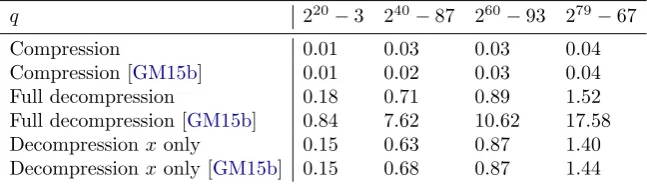
Comparison and Timings for g = 1, n = 3. We compare our method with the most effi-cient method from [GM15b] (there called “compression inti”) in terms of operations in Table1 and timings in Table2. We choose arbitrary elliptic curves such that the associated trace zero subgroups have prime order for fields of 20, 40, 60, and 79 bits. We see that the compression algorithm from [GM15b] requires fewer operations, but we could not observe a significant differ-ence in the timings (probably due to insufficient accuracy of our tests). For the decompression algorithm, we compare “full decompression”, where one entire point (including they-coordinate) is recomputed. Here, the method of [GM15b] is much slower (roughly by a factor 10), due to the necessary square root extraction. This shows one major efficiency advantage of the approach that we follow in this paper: Recovering the y-coordinate is much faster, since no square root computation is necessary. For a different point of view, we also compare “decompression inx
only”, where noy-coordinate is computed. In this case, the algorithm proposed in this paper and the one from [GM15b] behave similarly.
Table 1. Number of operations in Fq for compression/decompression of one point wheng= 1, n= 3
Compression 2S+6M+1I
Compression [GM15b] 1M
Full decompression 5S+5M+1I, 1 square root, 2 cube roots
Full decompression [GM15b] 4S+3M+2I, 1 square root, 2 cube roots, and 1 square root inFq3 Decompressionxonly 5S+4M+1I, 1 square root, 2 cube roots
Decompressionxonly [GM15b] 4S+3M+2I, 1 square root, 2 cube roots
Table 2. Average time in milliseconds for compression/decompression of one point wheng= 1, n= 3
q 220−3 240−87 260−93 279−67
Compression 0.01 0.03 0.03 0.04
Compression [GM15b] 0.01 0.02 0.03 0.04
Full decompression 0.18 0.71 0.89 1.52
Full decompression [GM15b] 0.84 7.62 10.62 17.58
Decompressionxonly 0.15 0.63 0.87 1.40
Decompressionxonly [GM15b] 0.15 0.68 0.87 1.44
Naumann [Nau99] does not give explicit compression or decompression algorithms, but he derives an equation for the trace zero subgroup that might be used for such. The equation is in the Weil restriction coordinates x0, x1, x2 of the x-coordinate of a trace zero point, and it has
degree 4 in x0 and degree 3 in x1, x2. Therefore, it allows a representation in the coordinates
(x0, x1) or (x0, x2), where decompression could be done by factoring a cubic polynomial in the
missing coordinate, and then recomputing the y-coordinate as a square root. Again, this is clearly more expensive than the decompression algorithm in this paper.
Comparison and Timings for g= 1, n= 5. A similar comparison for extension degree 5 (see Tables3and4) shows that the compression algorithm proposed in this paper is less efficient than that of [GM15b], but the decompression algorithm is faster. Although the bulk of the work in both decompression algorithms is polynomial factorization, following the approach proposed in this paper we have to factor one polynomial of degree 5 overFq5, where the algorithm of [GM15b] first factors a polynomial of degree 6 overFq, and then at least one polynomial of degree 5 over Fq5. For this reason, the decompression algorithm proposed in this paper performs better than that of [GM15b], regardless of whether we include the recovery of they-coordinate. Notice that we again compare with the best method from [GM15b], there called “compression/decompression in thesi with polynomial factorization”.
In comparison to [Sil05], our compression algorithm is less efficient, but our decompression method is more efficient. The decompression algorithm of Silverberg involves resultant computa-tions and the factorization of a degree 27 polynomial. If one wishes to recover they-coordinate, a square root extraction is also required. With or withour square root extraction, this is much more expensive than the decompression algorithm in this paper, which does not require poly-nomial factorization or resultant computations. We refer to [GM15b, Section 6] for a detailed analysis of the algorithm from [Sil05].
Table 3. Number of operations/complexity for compression/decompression of
one point wheng= 1, n= 5
Compression 3S+18M+3I inFq5
Compression [GM15b] 5S+13M in Fq
Full decompression O(logq) operations inFq
Full decompression [GM15b] O(logq) operations inFq, and 1 square root inFq5 Decompressionxonly O(logq) operations inFq
Decompressionxonly [GM15b] O(logq) operations inFq
Table 4. Average time in milliseconds for compression/decompression of one
point wheng= 1, n= 5
q 210−3 220−5 230−173 240−195
Compression 0.21 0.25 0.46 0.80
Compression [GM15b] 0.04 0.04 0.05 0.10
Full decompression 0.82 9.39 4.26 10.13
Full decompression [GM15b] 5.89 17.90 30.21 63.60
Decompressionxonly 0.77 9.36 4.01 9.82
Decompressionxonly [GM15b] 5.53 16.48 21.42 45.08
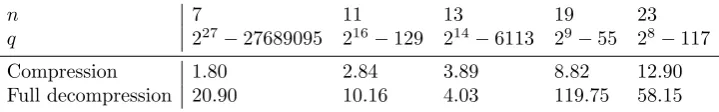
Table 5. Average time in milliseconds for compression/decompression of one point wheng= 1, n >5, log2|Tn| ≈160
n 7 11 13 19 23
q 227−27689095 216−129 214−6113 29−55 28−117
Compression 1.80 2.84 3.89 8.82 12.90
Full decompression 20.90 10.16 4.03 119.75 58.15
give in Table 5 timings for n = 7,11,13,19,23 and corresponding randomly chosen values of
q, A, andBthat produce prime order trace zero subgroups of approximately 160 bits. From the different values for decompression times (due to the fact that the performance of the polynomial factorization algorithm in Magma depends heavily on the specific choice ofqandn), we see that there is much room for optimization in the choice of these parameters.
In each case, we choose the fastest method of computinghP during compression. According to our experiments, this is an iterative approach forn= 7, a divide and conquer approach for
n= 11,13,19, and Algorithm7 forn≥23. During decompression we compute they-coordinate of the point as well, since the difference with computing thex-coordinate only is negligible.
We also report that we are able to apply our method to much larger trace zero subgroups and much larger values of n. More specifically, our implementation was tested on trace zero subgroups of more than 3000 bits and for values ofnlarger than 300. For even larger values of
n, the limitation is not our compression/decompression approach, but rather the fact that the trace zero subgroup becomes very large, even for small fields.
Table 6. Average time in milliseconds for compression/decompression of one
point wheng= 2, n= 3
q 25−1 28−75 210−3 213−2401 215−19
Compression 0.10 0.11 0.19 0.19 0.17
Full decompression 0.28 4.78 19.87 3.07 3.82
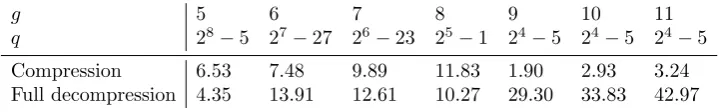
Table 7. Average time in milliseconds for compression/decompression of one point whenn= 5, g≥5, log2|Tn| ≈160
g 5 6 7 8 9 10 11
q 28−5 27−27 26−23 25−1 24−5 24−5 24−5
Compression 6.53 7.48 9.89 11.83 1.90 2.93 3.24
Full decompression 4.35 13.91 12.61 10.27 29.30 33.83 42.97
serves mostly as a proof of concept and for comparison purposes, we did not put much effort into producing suitable curves for larger trace zero subgroups.
The representation of [Lan04] consists of 4 (out of 6) Weil restriction coordinates of the coef-ficients of theu-polynomial of a point, plus two small numbers to resolve ambiguity. Following the notation of the original paper, we call the transmitted coordinatesu12, u11, u10, u02, the two small numbersa, b, and the dropped coordinates u01, u00. This approach requires as a precom-putation the elimination of 4 variables from a system of 6 equations of degree 3 in 10 variables. The result is a triangular system of 2 equations in 6 indeterminates. The compression algo-rithm substitutes the values of u12, u11, u10, u02 into the system and solves for the two missing values in order to determine a, b, which in turn determine the roots coinciding with u01, u00. The decompression algorithm uses a, b to decide which among the solutions of the system are the coordinates it recovers. The advantage of this algorithm is that it works entirely over Fq. Nevertheless, compression is clearly less efficient than our compression algorithm, since we only need to evaluate a number of expressions, while Lange has to solve a triangular system, which involves computing roots. While our decompression algorithm requires the factorization of one or two polynomials, which has complexity O(logq), Lange’s decompression algorithm solves again the same triangular system. Since this involves computing roots in Fq, which has complexity
O(log4q) using standard methods (and can be as low as O(log2q) for special choices of param-eters, see [BV06]), it is less efficient than the decompression algorithm proposed in this paper. Notice also that Lange’s approach does not give thev-polynomial, which needs to be computed separately, adding to the complexity of decompression.
Timings for g >2, n >3. As a proof of concept, we provide timings in Table7 for trace zero subgroups of approximately 160 bits whenn= 5 andg= 5,6, . . . ,11. The reason for this choice is simply that we are able to find suitable curves for these parameters. We stress again that the limitation here is not our compression method, but finding trace zero subgroups of known group order, so we expect that our method will work for much larger values ofnandg(e.g. we are able to compute an example forg= 2, n= 23, where the group has 173 bits).
6. Conclusion
representation has convenient mathematical properties: It identifies well-defined classes of points, it is compatible with scalar multiplication, and it does not discard the v-polynomial of the Mumford representation (or the y-coordinate of an elliptic curve point), thus saving expensive square root computations in the decompression process.
Our compression and decompression algorithms are efficient, even for medium to large values ofnandg. For those parameters where other compression methods are available (namely, for very smallnandg), our algorithms are comparable with or more efficient than the previously known ones, if compression and decompression are considered together. No costly precomputation is required during the setup of the system.
References
[AC07] R. M. Avanzi and E. Cesena,Trace zero varieties over fields of characteristic 2 for cryptographic applications, Proceedings of the First Symposium on Algebraic Geometry and Its Applications (SAGA ’07), 2007, pp. 188–215.
[ACD+06] R. Avanzi, H. Cohen, C. Doche, G. Frey, T. Lange, K. Nguyen, and F. Vercauteren,Handbook of elliptic and hyperelliptic curve cryptography, Discrete Mathematics and its Applications, Chapman & Hall/CRC, Boca Raton, 2006.
[BCHL13] J. W. Bos, C. Costello, H. Hisil, and K. Lauter, High-performance scalar multiplication using 8-dimensional GLV/GLS decomposition, Cryptographic Hardware and Embedded Systems – CHES 2013 (G. Bertoni and J.-S. Coron, eds.), LNCS, vol. 8086, Springer, 2013, pp. 331–338.
[BCP97] W. Bosma, J. Cannon, and C. Playoust, The Magma algebra system. I. The user language, J. Symbolic Comput.24(1997), 235–265.
[BDL+12] D. J. Bernstein, N. Duif, T. Lange, P. Schwabe, and B.-Y. Yang,High-speed high-security signatures,
J. Cryptogr. Eng.2(2012), no. 2, 77–89.
[Bla02] G. Blady,Die Weil-Restriktion elliptischer Kurven in der Kryptographie, Master’s thesis, Universit¨at GHS Essen, 2002.
[BV06] P. S. L. M. Barreto and J. S. Voloch, Efficient computation of roots in finite fields, Des. Codes Crytogr.39(2006), no. 2, 275–280.
[Can87] D. G. Cantor,Computing in the Jacobian of a hyperelliptic curve, Math. Comp.48(1987), no. 177, 95–101.
[Ces08] E. Cesena, Pairing with supersingular trace zero varieties revisited, Available at http://eprint. iacr.org/2008/404, 2008.
[Ces10] ,Trace zero varieties in pairing-based cryptography, Ph.D. thesis, Universit`a degli studi Roma Tre, Available athttp://ricerca.mat.uniroma3.it/dottorato/Tesi/tesicesena.pdf, 2010. [Die03] C. Diem,The GHS attack in odd characteristic, Ramanujan Math. Soc.18(2003), no. 1, 1–32. [Die11] ,On the discrete logarithm problem in class groups of curves, Math. Comp.80(2011), 443–
475.
[DS] C. Diem and J. Scholten, An attack on a trace-zero cryptosystem, Available athttp://www.math. uni-leipzig.de/diem/preprints.
[EGO11] P. N. J. Eagle, S. D. Galbraith, and J. Ong, Point compression for Koblitz curves, Adv. Math. Commun.5(2011), no. 1, 1–10.
[EGT11] A. Enge, P. Gaudry, and E. Thom´e,AnL(1/3)discrete logarithm algorithm for low degree curves, J. Cryptology24(2011), 24–41.
[FHLS14] A. Faz-Hern´andez, P. Longa, and A. H. S´anchez,Efficient and secure algorithms for GLV-based scalar multiplication and their implementation on GLV-GLS curves, Topics in cryptology CT-RSA 2014, LNCS, vol. 8366, Springer, 2014, pp. 1–27.
[Fre99] G. Frey, Applications of arithmetical geometry to cryptographic constructions, Proceedings of the 5th International Conference on Finite Fields and Applications, Springer, 1999, pp. 128–161. [Gau07] P. Gaudry,Fast genus 2 arithmetic based on Theta functions, J. Math. Cryptol.1(2007), 243–265. [Gau09] ,Index calculus for abelian varieties of small dimension and the elliptic curve discrete
loga-rithm problem, J. Symbolic Comput.44(2009), no. 12, 1690–1702.
[GH99] G. Gong and L. Harn,Public-key cryptosystems based on cubic finite field extensions, IEEE Trans. Inform. Theory45(1999), no. 7, 2601–2605.