On the Multi-output Filtering Model and Its Applications

(1)

Applications

Guang Gong, Kalikinkar Mandal, Yin Tan and Teng Wu

Department of Electrical and Computer Engineering University of Waterloo, Canada

{ggong,kmandal,y24tan,teng.wu}@uwaterloo.ca

Abstract. In this paper, we propose a novel technique, called multi-output filtering model, to study the non-randomness property of a cryptographic algorithm such as message authentication codes and block ciphers. A multi-output filtering model consists of a linear feedback shift register (LFSR) and a multi-output filtering function. Our contribution in this paper is twofold. First, we propose an attack technique under IND-CPA using the multi-output filtering model. By introducing a distinguishing function, we theoretically determine the success rate of this attack. In particular, we construct a distinguishing function based on the distribution of the linear complexity of component sequences, and apply it on studying TUAK’s f1 algorithm, AES, KASUMI and PRESENT. We demonstrate

that the success rate of the attack onKASUMI and PRESENT is non-negligible, but f1 and AES

are resistant to this attack. Second, we study the distribution of the cryptographic properties of component functions of a random primitive in the multi-output filtering model. Our experiments show some non-randomness in the distribution of algebraic degree and nonlinearity forKASUMI.

1 Introduction

LetC be a cryptographic scheme (keyed or non-keyed) with n-bit input and m-bit output. Clearly it can be simply regarded as a vectorial Boolean function from _Fn

2 to Fm2 . WhenC involves a key K, we should write CK for strictness, but we prefer to use C for simplicity if the context is clear. In most circumstances, the cryptographic properties of C, such as algebraic degree and nonlinearity, are difficult to be exploited due to the large values of n and m. A natural idea to overcome this difficulty is to restrict the inputs of C on a subspace S of _Fn

2. For instance, the subspace S can be generated by an `-stage linear feedback shift register (LFSR). Then we obtain a function C0 _from _S _{to its image set}

C(S). By adapting the size of S, we can study the cryptographic properties of C0_{. If} _C has good randomness properties, it should be difficult to find a subspace S such that C0 has bad randomness properties. We must mention that the above method for analyzing the cryptographic scheme C lies in a more general notion called subset cryptanalysis [27], which tries to track the statistical evolution of a certain subset of values through various operations in the cryptographic schemes. One is referred to [17] for a successful application of the subset cryptanalysis to find a 5-round collision on Keccak [5].

(2)

found in Section 3. We should mention that in this paper we restrict C to MACs and block ciphers, but this model can also be generalized to study other cryptographic primitives.

Thanks to the fruitful research outcome on the theory of sequences and Boolean func-tions, we can study the distribution of certain properties of the component sequences and functions. Such properties include linear complexity of the component sequences, algebraic degree and nonlinearity of the component functions, etc. Before describing our contribution in further, let us first briefly introduce the cryptographic primitives on which we apply the multi-output filtering model, especially on the recently proposedf1 algorithm of theTUAK algorithm set [41] for the 3rd _{Generation Partnership Project.}

TUAK is proposed to the 3rd _{Generation Partnership Project (3GPP) for providing} authenticity and key derivation functionalities in mobile communications. The design of TUAK is based on the Keccak permutation with 1600-bit internal state due to its good attack resistance property and its simple and efficient constructions of message authenti-cation code and key derivation function. The TUAKalgorithm set contains seven different algorithms, namely f1 to f5 and f1∗ and f5∗. The f1 ( or f1∗ as re-synchronisation message authentication) algorithm ensures the authenticity of messages, f2 is used for generating responses andf3 tof5 and f5∗ are used as key derivation functions. SinceTUAK’s design is closely based onKeccak’s design, one may expect that the security property ofTUAKmay inherit from that ofKeccak. The security evaluation forTUAKis essential for guaranteeing the authenticity in mobile communications. The details ofTUAKcan be found in Appendix A. The analysis of the resistance of TUAK to many known attacks has been presented in [22]. In this paper, we restrict ourselves to the analysis of the MAC generation algorithm f1 in the multi-output filtering model. Our analysis also considers the block ciphers AES [11], KASUMI [40], and PRESENT [8].

In Section 5, we introduce a generic distinguishing attack framework on C under the indistinguishability under chosen-plaintext attack model (IND-CPA for short), which is a variant of indistinguishability of encryptions proposed by Goldwasser and Micali [19] in public-key cryptography settings. This attack makes use of a special object, called a distin-guishing function. We theoretically determine the success rate of the attack. In particular, we construct a new type of distinguishing function by relying on the distribution of the linear complexity of the component sequences. Applying this new distinguishing function on f1, AES, KASUMI and PRESENT, we can distinguish the output of both KASUMI and PRESENT with the output of a random primitive with non-negligible success rate. On the other hand, our study shows that f1 and AES is immune to this attack.

Furthermore, in Section 6, we study the distribution of the algebraic degree and nonlin-earity of the component functions. We first determine the distribution of these two proper-ties for the component functions of a random multi-output filtering function. By performing experiments onf1,AES,KASUMIand PRESENT, it can be seen that, forKASUMI, the den-sity of its component functions with algebraic degree less than ` −2 is greater than the random case, where ` is the length of the LFSR. While the degree distributions of the other primitives are similar to that of the random case. This can be a potential risk of the security ofKASUMI when an adversary uses the decoding method of Reed-Muller code.

(3)

the algebraic degree and the nonlinearity of component functions off1and other primitives. Section 7 concludes our work.

2 Preliminaries

In this section, we provide some definitions and results that will be used in this paper. We first give a list of notations that we use throughout the paper.

Notations

- _F2: the Galois field with two elements{0,1};

- _F2n: a finite field with 2n elements that is defined by a primitive element α;

- _Fn

2: a vector space with 2n elements and each element is a binary n-tuple; - d(f): the algebraic degree of a Boolean functionf;

- NL(f): the nonlinearity of a Boolean function;

- LC(s): the linear complexity of a binary sequences with period N; - Π: Keccak-f[1600] permutation.

- Bn: the set of all Boolean functions with n variables.

2.1 Basic definitions on sequences

We present some definitions on sequences. For a well-rounded treatment of sequences and Boolean functions, the reader is referred to [10,21].

Let s={si}be a sequence generated by a linear feedback shift register (LFSR) whose recurrence relation is defined as

s`+i = `−1

X

j=0

cjsi+j, si, ci ∈F2, i= 0,1, ... (1)

where p(x) = `

P

i=1

cixi ∈ F2[x] is the characteristic polynomial of degree ` of the LFSR. A binary sequence s in Eq. (1) with period 2` ₋_{1 generated by an LFSR is called an} _m

-sequence. Let s={si} be an m-sequence of period 2`−1 and f(x0, ..., x`−1) be a Boolean function in ` variables. We define a sequence a={ai} as

ai =f(sr1+i, sr2+i, ..., srt+i), si, ai ∈F2, i≥0

where r1 < r2 < . . . < rt < ` are tap positions. Then the sequence a is called a filtering

sequence and the period of a equals 2`−1.

Thelinear complexityorlinear spanof a sequence is defined as the length of the shortest LFSR that generates the sequence. For an m-sequence, the linear complexity of an m -sequence is equal to the length of its LFSR [21]. On the other hand, the linear complexity of a nonlinear filtering sequence lies in the range of `and 2`₋_{1 [24]. If a filtering sequence} has linear complexity 2`−1, then we call it hasoptimal linear complexity.

2.2 Basic definitions on Boolean functions

(4)

Definition 1. Let f be a Boolean function from _Fn₂ to _F2. Then f can be uniquely

repre-sented by its algebraic normal form (ANF) as

f(x) = X

I∈P({0,...,n−1}) aIxI,

where aI ∈ F2, xI =

Q

i∈Ixi and P({0, . . . , n−1}) is the power set of {0, . . . , n−1}. The

algebraic degree of f, denoted by d(f), is the maximal size of I in the ANF of f such that

aI 6= 0.

One of the most important properties of Boolean functions is its nonlinearity, which was proposed to measure the distance of it to all affine functions. A cryptographic strong Boolean function is supposed to have high nonlinearity to resist linear attacks [29].

Definition 2. The Walsh spectrum of a Boolean functionf to a point a∈_Fn

2, denoted by Wf(a), is defined by

Wf(a) =

X

x∈_Fn

2

(−1)f(x)+a·x

where a·x is the inner product of a and x.

The nonlinearity of f can be defined in terms of the Walsh spectrum as

NL(f) = 2n−1−max a∈Fn2

|Wf(a)|

2 .

Whenn is an even positive integer, it is known that the maximum value if the nonlinearity of a Boolean function f is NL(f)≥2n−1−2n/2−1 [10]. A Boolean functions achieving this bound is called a bent function.

Let m and n be two positive integers. A function F, from _Fn

2 to Fm2 , defined by F(x) = (f1(x), f2(x), ..., fm(x)) is called a (n, m)-function, multi-output Boolean functions, or vectorial Boolean functions, where fi’s are called coordinate functions [10].

3 Multi-Output Filtering Model

In this section, we provide a detailed description of the multi-output filtering model of a cryptographic primitive.

3.1 Description of the multi-output filtering model

Leta={ai}i≥0 be a binary sequence generated by an `-stage linear feedback shift register (LFSR) whose recurrence relation is

a`+i = `−1

X

j=0

cjai+j, cj ∈F2, i≥0, (2)

where p(x) =x` ₊P`−1

i=0cix

i _{is a primitive polynomial of degree} _` _over

F2 and STATEj = (aj, aj+1, ..., a`−1+j) is called the j-th state of the LFSR. Using this LFSR, from the above sequence a, we generate a set of messages of n bits as follows R ={Rj : 0 ≤j ≤ 2`−2} where

(5)

where modulo 2`−1 is taken over the indices ofai’s. Note that the elements inRare in the sequential order. We now define the multi-output filtering model onF :{0,1}k_{× {}₀_,₁_}n _→

{0,1}m_{. For a fixed key K and for each R}

j with 0≤j ≤2`−2, we obtain Cj=F(K,Rj)

= (g0(K,Rj), . . . , gm−1(K,Rj))

,(yj,0, yj,1, . . . , yj,m−1).

(4)

Using a matrix, we can represent the above Cj as

    

C0 C1 .. . C₂`₋₂

    

=

    

y0,0 y0,1 · · · y0,m−1

y1,0 y1,1 · · · y1,m−1

..

. ... ...

y₂`_−2,0y₂`_−2,1· · · y₂`_−2,m−1

    

. (5)

The matrix (5) provides us two methods to study cryptographic properties of F as described below.

I. Sequence point of view:Each column in the above can be considered as a sequence of period 2`₋_{1 for a nonzero initial state of the LFSR. Each sequence of period 2}`₋₁ is called a component sequence. We denote the i-th component sequence by si and

si ={y0,i, y1,i, ..., y2`_−2,i}. s_i can also be considered as a filtering sequence with filter

function gi, 0≤i≤m−1.

II. Boolean function point of view: From (4) and (5), we see the following process

gi :

STATEj ∈F`2 of the LFSR → {Rj ∈Fn2} →i-th component sequence.

Therefore, each component sequence can also be regarded as a Boolean function on

F`2. Note that, for a nonzero initial state, the LFSR cannot generate all-zero state, we need to query F to get the output valueF(K,0n_{) for all-zero input for all component} Boolean functions. With a fixed K inF, using an`-stage LFSR, we obtain mBoolean functions on _F`₂. Mathematically, m Boolean functions gi :F2` →_F₂ (0≤i≤m−1)

are defined as

gi(K,STATEj) = yj,i, (0≤j ≤2`−2). (6) We call each Boolean function gi acomponent orcoordinate function of F.

3.2 Application to TUAK’s f1,AES, KASUMI and PRESENT

For the sake of clarity on the input assignment, we briefly explain how we apply the multi-output filtering model on TUAK’s f1, and block ciphersAES, PRESENT and KASUMI.

TUAK’s f1: Recall that f1 takes K, RAND, and SQN as inputs. Now we fix a key K and a sequence number SQN. We use an `-stage LFSR to generate random numbers RANDj in f1. Denoting by the i-th state of the `-stage LFSR by STATEi ∈F`2. We obtain 2`−1 different n-bit RAND numbers R ={Rj : 0≤ j ≤ 2`−2} by Eq. (3) and the component sequences and component functions are obtained using Eq. (4) with Cj =f1(K,Rj,SQN).

Remark 1. For TUAK’s f1 function, in Eq. (5), recovering the last bit y2`_−2,i for each

component sequence si from the previous 2`−2 bits is equivalent to recoveringC2`₋₂ from

(6)

AES,PRESENTand KASUMI: Recall thatAES 128 accepts a 128-bit key and a 128-bit input and produces an output of 128 bits, andAES 256 accepts a 256-bit key and a 128-bit input and produces an output of 128 bits [11].KASUMIhas a 64-bit input, a 128-bit key, and a 64-bit output. For AES 128 andAES 256, the inputs messages of 128 bits are generated using an LFSR of length`and by Eq. (3), and the component sequences and functions are obtained using Eq. (4) with Cj = AES 128 (K,Rj) and Cj = AES 256 (K,Rj). PRESENT [8] is a 64-bit block cipher with a 80-bit key. The component sequences and functions of PRESENT are obtained using Eq. (4) with Cj = PRESENT(K,Rj). KASUMI [40] is a 64-bit block cipher with a 128-64-bit key. The 64-64-bit inputs messages are generated by Eq. (3) with n = 64 and the component sequences and functions are obtained using Eq. (4) with Cj =KASUMI(K,Rj).

4 Distinguishing Attack Model

In this section, we describe the attack model of our distinguishing attack on a message authentication code and a block cipher. In this paper we restrict ourselves to message authentication codes and block ciphers. The attack model is based on indistinguishability (IND) of encryptions under chosen-plaintext attack (CPA) (IND-CPA), which was first de-veloped due to Goldwasser and Micali [19] in public-key settings. In [3], Bellareet al. stud-ied the indistinguishability of encryptions under chosen-plaintext attack in the symmetric key setting. Here, we use the same attack model to distinguish MACs (or ciphertexts) in the symmetric-key setting. However, we develop a new distinguishing technique based on linear complexity of component sequences in the multi-output filtering model for deciding the MAC (or ciphertext). For the message authentication code, the aim of an adversary is to distinguish two MACs for two messages P0 and P1 with a high probability where messages P0 and P1 were chosen by the adversary. On the other hand, for an encryption, the adversary aims at distinguishing two ciphertexts for two chosen messages P0 and P1 with a high probability.

Let F : {0,1}k _{× {}₀_,₁_}n _{→ {}₀_,₁_}m _{be a cryptographic algorithm which accepts two} inputs, a key of length k and a message of length n and produces an output of length m. Assume that P0 and P1 are two messages of length n chosen by the adversary, the length of the key K is k and ci = F(K, Pi), i = 0,1. The aim of the distinguishing attack is to distinguish c0 and c1 for the messages P0 and P1 with high probability. We denote the random oracle by O and the adversary byA. The indistinguishability game [2,19] between the random oracle and the adversary is played as follows.

(1) Fixing a key K and generating the set of messages R = {R0, R1, ..., RN−1} using an LFSR with a primitive polynomial of degree `,N = 2`−1;

(2) The adversary A randomly picks up P0 ∈ R and P1 6∈ R and sends both {P0, P1} to

O.

(3) The random oracle picks up Pb $

←− {P0, P1},b = 0 or 1 and computesc=F(K, Pb).O sends c to the adversary A.

(4) Once A receives c as a challenge, the adversary performs a technique and decides b0 and returns b0 to O whereb0 = 0 or 1;

(5) If b=b0, then adversary A succeeds; otherwise she fails.

We also summarize the game in Figure 1.

(7)

AdversaryA Random oracleO R={R0, R1, . . . RN−1}

P0∈ R,P1 $

←− {0,1}n andP1∈ R/

{P0, P1}

−−−−−−−−−−−−→

b←− {$ 0,1}

c=F(K, Pb) c

←−−−−−−− Aapplies distinguishing functionh

to decideb0

b0

−−−−−−−→ Checkb

0 =?b Success ifb0=b

←−−−−−−−−−−−

Fail ifb06=b

←−−−−−−−−

Fig. 1: Indistinguishability game

MACs produced byf1 forP0 and P1 with probability greater than 1/2. Therefore, the new method provides a construction of a distinguisher on f1.

5 Distinguishing Attack Based on Linear Complexity

In this section, we first present a general technique to build a distinguisher of a crypto-graphic primitive, followed by the theoretical determination of the success probability of the distinguishing attack. In particular, we make use of the distribution of the linear com-plexity of component sequences of a primitive to develop a new distinguisher. Finally we apply this technique on f1,AES, KASUMI, and PRESENT.

5.1 A generic framework to build a distinguisher

We start this section by the following definition.

Definition 3. Let R and S be two subsets of U, where S = U \ R. Let Ω be a subset

of R × S. Let C be a cryptographic scheme from U to some set V. For any P0 ∈ R and

P1 ∈ S, define a distinguishing function h : {C(P0),C(P1)} → {0,1}. We say that C is

distinguishable with respect to R,S, h, Ω if the average probability

X

i∈{0,1}

Prh(c) =i∧c=C(Pi)

is non-negligible compared with 1/2, when (P0, P1) is randomly chosen from Ω.

Now we state the main theorem below and provide the proof of it in Appendix B due to the page limit.

Theorem 1. Let the notations be the same as above. Now we define a subset CS of U, which is called the condition set. Let S0 _{⊂ S} _and _Ω ₌_{R × S}0_{. For any} _P

0 ∈ R, P1 ∈ S0,

let us define the distinguishing function h:{C(P0),C(P1)} → {0,1} as

h(y) =

(

0 if y=C(x) and x∈ CS,

(8)

Define the following two probabilities

q0= Pr (x0 ∈ R ∧x0 ∈ CS), q1= Pr (x1 ∈ S0∧x1 ∈ CS).

(8)

where (x0, x1) $

←−Ω. Then the average probability is

X

i∈{0,1}

Pr (h(c) =i∧c=C(Pi) ) =

1 + (q0−q1)

2 . (9)

Several remarks on Theorem 1 are as follows:

(i) An attacker will expect the probability value in (9) to be as large as possible so that she can distinguish the cryptographic schemeC with a high probability.

(ii) The difficulty of finding the distinguishing attack described in Theorem 1 is to find a proper condition setCS such thatq0−q1 is large.

(iii) The value of q0−q1 could be negative. If the attacker uses CS to replace CS, q0−q1 will be positive, and the probability will be greater than 0.5. Thus, the problem of finding a condition set such that q0−q1 is large becomes the problem of finding the condition set such that |q0−q1| is large.

(iv) In the rest of this section, we will show how to construct such setCS, which leads to distinguishing attack onKASUMI and PRESENT with non-negligible success rate.

5.2 Distribution of the linear complexity of component sequences

We use f1,AES,KASUMI and PRESENT as multi-output filtering functions and study the distribution of the linear complexities of their component sequences. Meidl and Niederreiter studied the expectation of the linear complexity of random binary periodic sequences in [30]. Unfortunately, the average values of the linear complexities of the component sequences of AES, f1, KASUMI, PRESENT are very close to the theoretical value determined in [30] according to our experiments. This motivates us to look at the whole distribution of the linear complexity of the component sequences instead of considering only the average value. We perform the following test for the linear complexity and have an interesting observation on the component sequences of KASUMI and PRESENT.

Test of the distribution of linear complexity. Usually, for a primitiveC, it is difficult to determine the distribution of linear complexity of its component sequences. Of course, one can choose a subset of inputs to the primitive to estimate the linear complexity dis-tribution. However, since the input space is very large, it is hard to measure the accuracy of the estimated distribution. To avoid such problem, we propose a new method to test the distribution. This goal is achieved by choosing two (large) subsets of inputs and by comparing the distributions of the linear complexity of their component sequences. In par-ticular, we choose one subset LI of the inputs to be generated by an `-stage LFSR and the other subset RI = (LI \ {P0})∪ {P1}, where P0

$

←− LI and P1

$

←− LI. Note that the elements in LI are ordered according to Eq. (3). It is clear that if the C has very good random property, it should not be easy to distinguish two distributions for LI and RI. Our method consists of the following three steps.

(9)

Step 1 (Generating component sequences). We randomly chooseNkey keys.

1. For all keys, using LI as the set of inputs and C as a multi-output filter, we obtain m·Nkey component sequences. This set of component sequences is denoted by Q1. 2. Similarly, using RI as the inputs, we generate another set of m · Nkey component

sequences, which is denoted by Q2.

Step 2 (Computing linear complexity). We compute the linear complexities of the

sequences in Q1 and Q2 and count the number of component sequences in Qi with the linear complexity 2`₋_{2 and 2}`₋_{1, denoted by} _Ni

2`₋₁ and N₂i`₋₂, wherei= 1 or 2.

Step 3 (Comparing the distributions). Now we compare two distributions by

com-puting the slopes sli of the line between two points (2` −2, N₂i`₋₂) and (2

` ₋₁_{, N}i 2`₋₁),

where

sli = Ni

2`₋₁−N₂i`₋₂

(2`₋₁₎₋₍₂`₋₂₎ =N i

2`₋₁−N₂i`₋₂.

If the difference between sl1 and sl2 is non-negligible, we can make use of it to build a distinguisher of C, which is described in the next section. The worst case computational complexity for exhausting all `-stage LFSRs of the above three steps is

φ(2`₋₁₎

` ×Nkey×2`×(2

`₋₁₎_×_m, ₍₁₀₎

where φ is the Euler phi function. We perform the experiment using these parameters on f1, AES, KASUMI and PRESENT in the next section.

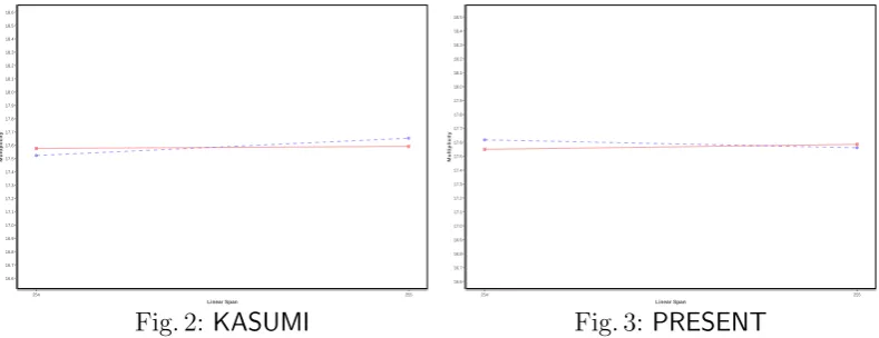
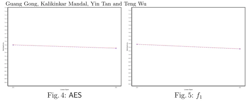
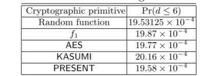
Distribution off1,AES,KASUMIandPRESENT. In our experiment, we choose`= 8

and Nkey = 108. By Eq. (10), the worst case complexity for the primitive f1 is 250.27 (some computation can be performed in a parallel way). We present the result in the following figures. In the figures, the red (resp. blue) line represents the distribution of sequences in Q1 (resp. Q2).

254 255 Linear Span 16.6 16.7 16.8 16.9 17.0 17.1 17.2 17.3 17.4 17.5 17.6 17.7 17.8 17.9 18.0 18.1 18.2 18.3 18.4 18.5 18.6 Multiplicity

Fig. 2: KASUMI

254 255 Linear Span 16.6 16.7 16.8 16.9 17.0 17.1 17.2 17.3 17.4 17.5 17.6 17.7 17.8 17.9 18.0 18.1 18.2 18.3 18.4 18.5 Multiplicity

(10)

Fig. 4: AES

Fig. 5: f1

From Figs. 2 and 3, one can observe that, for KASUMI and PRESENT, the difference of the distribution of the linear complexity for sequences in Q1 and Q2 is non-negligible. While Figs. 4 and 5 show this is not the case for AES and f1.

5.3 The new distinguishing attack

We now present the details of our distinguishing attack, which is achieved through con-structing a distinguishing function h. The construction of the distinguishing function is based on the linear complexity distribution of the component sequences of a primitive in the multi-output filtering model.

Constructing the distinguishing function. Recall that the distinguishing function is defined in Definition 3. We use the notations in Theorem 1 and the attack model is depicted in Fig. 1.

1. Choosing an`-stage LFSR with a primitive polynomial to generate the inputs of length n inR (see Eq. (3)). For f1 and AES,n = 128; forKASUMI and PRESENT, n= 64. 2. Constructing S =_Fn

2 \ R;

3. Randomly choose a message P0 ∈ R and P1 ∈ S;

4. Let NLC be the number of component sequences with linear complexity LC where ` ≤LC ≤2`−1;

5. Defining the condition set

CS =

  

y∈_Fn 2

using (R \ {P0})∪ {y}as the inputs of a primitive in the multi-output filtering model, the slope of the line between the points (2`₋₂_{, N}

2`₋₂) and (2`−1, N₂`₋₁) is less than t.

  

;

6. The distinguishing function h is defined in Eq. (7) using the condition setCS; 7. q0, q1 are the probability values defined in Definition 3.

5.4 An example of the attack

In this section, we apply the attack with our distinguishing function defined in Section 5.3 on f1, AES, KASUMI, and PRESENT. Theorem 1 and the observations in Figs. 2 and 3 enable us to gain a non-negligible success rate of the attack on KASUMI and PRESENT. For simplicity, we use an 8-stage LFSR to conduct our attack. However, one can use an arbitrary stage LFSR based on computation capability.

(11)

we use the distinguishing function h to execute the attack. It is worth to mention that, to test the average success rate is stable, we repeated the experiment 20 times by choosing different groups of 210 _{keys and found similar results for all experiments. Due to the page} limit, we present the average success rate for an experiment in Table 1, where we use the upper bound of the slopetand the 8-stage LFSR the same as those in Table 5 in Appendix C.

Table 1: Average success rate of our attack on f1,AES, KASUMI and PRESENT

Primitive t q0 q1 Avg. Succ. Rate

f1 2 0.20398 0.194458 50.476%

AES 2 0.193848 0.20044 50.329% KASUMI 4 0.421875 0.454103 51.612% PRESENT5 0.5686 0.540285 51.416%

One can observe from the average success rate in Table 1 that the outputs of both KASUMIandPRESENTcan be distinguished from a random primitive with a non-negligible probability. On the other hand, the performance off1 andAESis very similar to the random one.

6 Distribution of the Algebraic Degree and Nonlinearity of the

Component Functions

In this section, we investigate the distribution of the algebraic degree and the nonlinearity of the component functions of f1, AES,KASUMI, and PRESENT in the multi-output filtering model. To measure the randomness property, we first determine the distribution of the algebraic degree and the nonlinearity of component functions using a random primitive as the multi-output filter. Comparing this ideal distribution with those of f1, AES, KASUMI and PRESENT obtained by performing experiments, some non-randomness property of KASUMI is discovered. On the other hand, our experimental results show thatf1,AESand PRESENT perform very similar to the ideal case in the sense of the distributions of the algebraic degree and nonlinearity.

6.1 Algebraic degree distribution

Recall that the algebraic degree of a Boolean function is defined in Section 2. The following result states the number of Boolean functions with a given algebraic degree. The first part of the result can also be found in [10]. We provide a simple proof below for the completeness.

Theorem 2. Let f be a Boolean function on _F2n. Then the number of Boolean functions

with algebraic degree at most d is 2Pdi=0( n

i), and the number of Boolean functions with

algebraic degree exactly d is

2(nd)−1

2Pd−i=01(

n i)

Proof. Denoting the set Ω ={0,1, . . . , n−1}. Let the ANF off be f(x) = P

I∈P(Ω)aIxI. If the degree off is at mostd, then allaI = 0 for |I|> d. Clearly there are Pd_i=0 n_i

terms in the ANF of f with |I| ≤ d, and their coefficients can be either 0 or 1. Therefore there are 2Pdi=0(

n

i) Boolean functions with degree at mostd. For simplicity, let us denote by A

(12)

Corollary 1. LetC be a random cryptographic primitive andL be ann-stage LFSR whose characteristic polynomial is a primitive polynomial of degree n. We use C as a multi-output filtering function and L to generate the inputs of C. Then the probability of the component

functions having degree at most d is 2

Pd i=0(ni)

22n . In particular, Pr(d≤n−3) =

1 2n+1. Several remarks on the application of Theorem 2 are in the sequel:

(1) Assume the primitive C is used to generate MACs (for instance the function f1 in TUAK). If the percentage of component functions with degree less thann−2 is large, then we may use the decoding method of the Reed-Muller code R(n, n−3) to forge the MACs. See [28] for the Reed-Muller decoding. Note that the code R(n, n−3) is the set of Boolean functions on _F2n with algebraic degree at most n−3. Therefore, we

need the probability Pr(d≤n−3) to be as small as possible.

(2) On the other way, as shown in Corollary 1, for a random primitive, the probability Pr(d≤n−3) = ₂n1+1. So, for the primitive C, if this probability is very different with

1

2n+1, some non-randomness properties may be exploited.

(3) The probability Pr(d ≤ n −3) is actually affected by the diffusion property of the primitive C. Assumed C is a keyed primitive from _F2n to _F₂m. In the modern design

of ciphers, by increasing the number of iteration rounds, normally C could attain the maximal possible degree for any keyK. For a keyed primitiveCK, in the multi-output model, we restrict the inputs ofCK to a subspace S generated by an LFSR. For a fixed key K, CK can be regarded as a vectorial function and the ANF of CK has the form

CK(x) =

P

I∈P(Ω)aI(K)xI, where Ω ={0, . . . , n−1} and P(Ω) is the power set and aI(K) ∈ F2m are the coefficients of xI (a_I is a function with K as the variable) [10].

Then the restrictions of CK|S =P_{I∈P(Ω),I⊂S}aI(K)xI. The degree d of the component functions is then determined by aI with |I| = d. If the diffusion property of C and the key generating algorithm are good, it should be very rare that all aI = 0 for

|I| ≥dim(S)−2.

To better understand Theorem 2 and the above comments, for f1,AES,KASUMI and PRESENT, we perform the following test on the distribution of the algebraic degree of their component functions.

Statistical Test 1 By Corollary 1, using an LFSR with a primitive polynomial of degree 8, the probability that the degree of the component functions is smaller than 7 is ₂19 = 19.53125×10−4. For f1,AES,KASUMI and PRESENT, we apply the multi-output filtering

model as in Section 3.1. We choose 50,000keys for these primitives and compute the degree of the component functions. The probability of the degree is smaller than 7 is listed in the following table.

Table 2: Distribution of the degree smaller than 7

Cryptographic primitive Pr(d≤6) Random function 19.53125×10−4

f1 19.87×10−4

AES 19.77×10−4

KASUMI 20.16×10−4

PRESENT 19.58×10−4

(13)

probability is very close to it. This points out a distinguisher of KASUMI and other ciphers in Table 2.

6.2 Nonlinearity distribution

The nonlinearity of a Boolean function is one of the most important cryptographic prop-erties. A highly nonlinear function is used to avoid the linear attack and its variants. Let f be a Boolean function on _Fn₂. The nonlinearity of f is defined in Section 2. One can see easily from its definition that, in other words,

NL(f) = max

g∈RM(1,n)d(f, g),

where RM(1, n) denotes all Boolean functions with degree at most 1, and d(f, g) is the weight of the sequence (f(x) +g(x) :x∈_Fn

2). It is well known that when n is even the best nonlinearity a Boolean function may achieve is 2n−1−2n/2−1 and such functions are called bent functions (see [10] for more details). However, such functions are very rare. For a random Boolean function, we have the following result on the distribution of its nonlinearity.

Theorem 3 ([36,10]). Let c be any strictly positive real number. The density of the set

n

f ∈ Bn, NL(f)≥2n−1 −c

√

n2n−21

o

is greater than 1−2n+1−c2nlog2e. If c2log

2e >1, then this density tends to 1 whenn tends

to infinity.

Applying the above theorem on Boolean functions with 8 variables, we have the follow-ing table. Note that the best nonlinearity we expect for Boolean functions with 8 variables is 27 ₋₂3 _{= 120.}

Table 3: Lower bound of the density of Boolean functions in B8 with nonlinearity greater than W

Lower BoundW of NL Lower bound of the density of Boolean functions with NL(f)≥W 98 0.547478790614789878029979196008 97 0.719023101510754029847811117031 96 0.828242210249647874600628825765 95 0.896634306072499532736808245299 94 0.938757831567911386351203605713 93 0.964277746514500200807343273821 92 0.979486428025371618477752447455 91 0.988402673490240554092683405343 90 0.993545113167509528277258485524

(14)

Statistical Test 2 Let the LFSR and the other settings be the same as in Statistical Test 1. We list the distribution of the nonlinearity of the component functions of f1 and

AES in the following table. Since only the component functions with smallest nonlinearity are important to us (as an attacker), we only list the probability that a Boolean function has nonlinearity smaller than 90 or 91. The notationPr<W denotes the probability that the

nonlinearity is smaller than W.

Table 4: The distribution of the nonlinearity of component sequences of f1,AES,KASUMI and PRESENT

Cryptographic primitive Pr<90 Pr<91

Random Function 0.006455 0.011597 f1 0.000299 0.000690

AES 0.000306 0.000592 KASUMI 0.000299 0.000565 PRESENT 0.000308 0.000589

Unlike the distribution of the algebraic degree, from the above table we can not see obvious difference among these four ciphers. However, one can still see that the probability values Pr<90 and Pr<91 is still very different with the random case (although they are only

the upper bounds of the probability).

Although now we cannot derive attacks from Statistical Test 1 and Statistical Test 2, it is interesting to observe some non-randomness in the aspect of the distribution of cryp-tographic properties.

7 Concluding Remarks and Future Work

In this paper, we introduced the multi-output filtering model for analyzing the security of a cryptographic primitive. In this model, a cryptographic primitive is used as a multi-output filtering function and a number of component sequences and component functions of the primitive are obtained. We aimed at exploiting the security properties of the primitive through studying its component sequences and functions.

Thanks to the fruitful research outcome in the theory of sequences and Boolean func-tions, we propose a general distinguish attack technique under IND-CPA. We developed a new object, called a distinguishing function, to characterize the success rate of our new attack method. Interestingly enough, for a primitive C, by comparing the distribution of the linear complexity of the component sequences generated by two sets of inputs, we can construct a new distinguishing function. The importance of this new distinguishing func-tion is demonstrated by launching an attack onKASUMIandPRESENTwith non-negligible success rates.

Furthermore, we studied the cryptographic properties of the component functions. By comparing the distribution of the algebraic degree and nonlinearity properties with that of a random one, we discovered that, for KASUMI, its distribution of the algebraic degree is very different, while the distribution of f1, AES and PRESENT is not. We cannot propose any immediate attack based on this observation, but it is interesting to point it out for future research.

(15)

and other properties of component sequences and functions. This study may lead to a new attacking method, and present new criteria on designing a cryptographic primitive.

References

1. Aumasson, J.-P., Meier, W.: Zero-sum distinguishers for deduced Keccak-f and for the core functions of Luffa and Hamsi. Presented at the rump session of CHES 2009 (2009)

2. Bellare, M., Desai, A., Pointcheval, D., Rogaway, P.: Relations among notions of security for public-key encryp-tion schemes. Advances in Cryptology CRYPTO ’98, LNCS, vol. 1462, pp. 26 – 45. Springer Berlin Heidelberg (1998)

3. Bellare, M., Desai, A., Jokipii E., Rogaway, P.: A concrete security treatment of symmetric encryption: Analysis of the DES modes of operation. Proceedings of the 38th Symposium on Foundations of Computer Science, IEEE (1997)

4. Bernstein, D.J.: Second preimages for 6 (7? (8??)) rounds of Keccak?. http://ehash.iaik.tugraz.at/ uploads/6/65/NIST-mailing-list_Bernstein-Daemen.txt(2010)

5. Bertoni, G., Daemen, J., Peeters, M., Assche G.V.: The Keccak reference. http://keccak.noekeon.org/ Keccak-reference-3.0.pdf(2011)

6. Bertoni, G., Daemen, J., Peeters, M., Van Assche, G.: Cryptographic sponge functions, January 2011, http://sponge.noekeon.org/.

7. Bertoni, G., Daemen, J., Peeters, M., Van Assche, G.: Keccak sponge function family main document, submis-sion to NIST (updated), Versubmis-sion 1.2, 2009.

8. Bogdanov, A., Knudsen, L.R., Leander, G. Paar, C., Poschmann, A., Robshaw, M.J.B., Seurin, Y., Vikkelsoe, C.: PRESENT: An ultra-lightweight block cipher, Cryptographic Hardware and Embedded Systems - CHES 2007, LNCS, vol. 4727, pp. 450 – 466. Springer Berlin Heidelberg (2007)

9. Boura, C., Canteaut, A.: Zero-sum distinguishers for iterated permutations and application to Keccak-f and Hamsi-256. In: Biryukov, A., Gong, G., Stinson, D.R. (eds.) SAC 2011. LNCS, vol. 6544, pp. 1 – 17. Springer-Heidelberg (2011)

10. Carlet, C.: Boolean functions for cryptography and error correcting codes, Chapter of the monography boolean models and methods in mathematics, computer science, and engineering, Cambridge University Press, Yves Crama and Peter L. Hammer (eds.), pp. 257-397. (2010)

11. Daemen, J., Rijmen, V.: The Design of Rijndael, AES – The Advanced Encryption Standard. Springer (2002) 12. Daemen, J., Van Assche, G.: Differential propagation analysis ofKeccak. Fast Software Encryption, FSE 2012.

LNCS, vol. 7549, pp. 422 – 441. Springer Berlin Heidelberg (2012)

13. Daemen, J.: Permutation-based encryption, authentication and authenticated encryption. DIAC (2012) 14. Dinur, I., Morawiecki, P., Pieprzyk, J., Srebrny, M., Straus, M.: Practical complexity cube attacks on

round-reduced Keccak sponge function. Cryptology ePrint Archive, Report 2014/259 (2014) http://eprint.iacr. org/

15. Dinur, I., Shamir, A.: Cube attacks on tweakable black box polynomials. Advances in Cryptology-EUROCRYPT ’09, LNCS, pp. 278–299. Springer-Verlag (2009)

16. Dinur, I., Dunkelman, O., Shamir, A.: New attacks on Keccak-224 and Keccak-256. In: Canteaut, A. (ed.) FSE 2012. LNCS, vol. 7549, pp. 442-461, Springer, Heidelberg (2012)

17. Dinur, I., Dunkelman, O., Shamir, A.: Collision attacks on up to 5 rounds of SHA-3 using generalized internal differentials. Cryptology ePrint Archive, Report 2012/627. (2012)http://eprint.iacr.org/

18. Duc, A., Guo, J., Peyrin, T., Wei, L., Unaligned rebound attack: Application to Keccak. In: Canteaut, A. (ed.) FSE 2012. LNCS, vol. 7549, pp. 402-421, Springer, Heidelberg (2012)

19. Goldwasser, S., Micali, S.: Probabilistic encryption. Journal of Computer and System Sciences 28, 270 – 299 (1984)

20. Golomb, S.W.: Register Sequences. Aegean Park Press, Laguna Hills, CA (1981)

21. Golomb, S.W., Gong, G.: Signal design for good correlation – for wireless communication, cryptography and radar. Cambridge Press, 2005.

22. Gong, G., Mandal, K., Tan, Y., Wu, T.: Security Assessment of TUAK Algorithm Set, 2014.

23. Homsirikamol, E., Morawiecki, P., Rogawski, M., Srebrny, M.: Security margin evaluation of SHA-3 contest finalists through sat-based attacks. In A. Cortesi, N. Chaki, K. Saeed, and S.T. Wierzchon, (eds.). CISIM, LNCS, vol. 7564, pp. 56 – 67. Springer (2012)

24. Key, E.L.: An analysis of the structure and complexity of nonlinear binary sequence generators. IEEE Trans-actions on Information Theory 22, 732 – 736. (1976)

25. Lai, X., Duan, M.: Improved zero-sum distinguisher for full round Keccak-f permutation. Cryptology ePrint Archive, Report 2011/023 (2011),http://eprint.iacr.org/2011/023

26. Lathrop, J.: Cube attacks on cryptographic hash functions [EB/OL], Master’s Thesis. (2009)http://www.cs. rit.edu/~jal6806/thesis/.

(16)

28. MacWilliams, F.J., Sloane, N.J.A.: The theory of error-correcting codes. North-Holland Mathematical Library. (1977)

29. Matsui, M.: Linear cryptanalysis method for DES cipher. EUROCRYPT ’93, LNCS vol. 765, pp. 55–64. (1994) 30. Meidl, W., Niederreiter, H.: On the expected value of the linear complexity and thek-error linear complexity

of periodic sequences. IEEE Transaction on Information Theory, 48(11) 2817–2825. (2002)

31. Menezes, A.J., van Oorschot, P.C., Vanstone, S.A.: Handbook of applied cryptography, CRC Press (1997) 32. Morawiecki, P., Pieprzyk, J., Srebrny M., Straus, M.: Preimage attacks on the round-reduced Keccak with the

aid of differential cryptanalysis, Cryptology ePrint Archive, Report 2013/561 (2013)http://eprint.iacr.org/ 33. Morawiecki, P., Pieprzyk, J., Srebrny, M.: Rotational cryptanalysis of round-reduced KECCAK, Cryptology

ePrint Archive, Report 2012/546. (2012) http://eprint.iacr.org/.

34. Naya-Plasencia, Røck, M.A., Meier, W.: Practical analysis of reduced-round Keccak. In: Bernstein, D.J., Chat-terjee, S. (eds.) INDOCRYPT 2011. LNCS, vol. 7107, pp. 236-254. Springer, Heidelberg (2011)

35. NIST, the SHA-3 competition (2007-2012).http://csrc.nist.gov/groups/ST/hash/sha-3/index.html 36. Olejar, D., Stanek, M.: On Cryptographic properties of random boolean functions. Journal of Universal

Com-puter Science, 4(8), 705 – 717. (1998)

37. Rueppel, R.A.: Analysis and design of stream ciphers. Springer-Verlag, Berlin (1986) 38. Uspensky, J.V.: Introduction to mathematical probability. New York McGraw-Hill (1937)

39. Tan, Y., Mandal, K., Gong, G.: Characterization of column parity kernel and differential cryptanalysis of Keecak. CACR 2014-01, University of Waterloo. (2014)http://cacr.uwaterloo.ca/.

40. 3rd generation partnership project, Technical specification group services and system aspects, 3G security, specification of the 3GPP confidentiality and integrity algorithms; Document 2: KASUMI specification, V.3.1.1, 2001.

41. Specification of the TUAK algorithm set: A second example algorithm set for the 3GPP authentication and key generation functionsf1, f1∗, f2, f3, f4, f5 andf5∗, SP-130602, ETSI/SAGE, Dec 13, 2013.http://www.3gpp.

org/ftp/tsg_sa/TSG_SA/TSGS_62/ftp-TdocsByTdoc_SP-62.htm

Appendix

Here we present a description of TUAK’s f1 algorithm, the proofs of Theorem 1, and the slope of the linear complexity distribution off1 and AES, KASUMI and PRESENT.

A: Overview of TUAK algorithm set

TheTUAKalgorithm set is designed to generate message authentication codes (MAC) and various keys such as cipher keys and integrity keys in mobile communications. The TUAK algorithm set consists of seven algorithms, namely f1, f1∗, f2, f3, f4, f5, f5∗, which are built upon the Keccak permutation Keccak-f[1600] [41]. Each algorithm in TUAK is used to perform some specific task, for instance f1 and f1∗ are used to generate MACs, f2 to f5 are used to output signed response (RES), confidentiality key (CK), integrity key (IK), anonymity key (AK), respectively. The MAC and various keys are expected to guarantee the security in mobile communications.

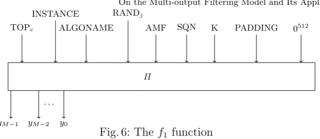
Description of f1

(17)

Π TOPc

INSTANCE

ALGONAME RANDj

AMF SQN K PADDING 0512

yM−1 yM−2

· · ·

y0

Fig. 6: Thef1 function Mathematically, we can write f1 in the form:

f1 ,Π(INPUT) = (y0, y1· · · , yM−1), (11)

where M is the length of the MAC and INPUT is defined as

INPUT =TOPc||INSTANCE||ALGORITHM||K||RAND||AMF||SQN||PADDING||0512. (12)

Note that, in the INPUT, except K, RAND, SQN, the other parameters are all prescribed constants. For details, see [41]. For the convenience, in the rest of the paper, we write f1 as

f1(K,RAND,SQN) = (y0, y1· · · , yM−1).

The algorithm f1 is flexible with the length of the parameters. The key length is 128 or 256 bits, the length of RAND is 128 bits, the length of SQN is 48 bits, and the possible output lengths are 64, 128, and 256.

B: Proof of Theorem 1

We present the proof of Theorem 1 below.

Proof. It is not difficult to see that there are four independent cases of the event h(c) = i∧c=C(Pi) when i ∈ {0,1}, theorefore we may compute its probability one by one and sum them together:

(1). h(c) = 0∧c=C(P0)∧P0 ∈ CS. The probability of this case equals

Pr (h(c) = 0 |c=C(P0)∧P0 ∈ CS ) Pr (c=C(P0)|P0 ∈P ) Pr (P0 ∈ CS ) = 1 2q0; (2). h(c) = 0∧c=C(P0)∧P0 6∈ CS. The probability of this case is clear 0.

(3). h(c) = 1∧c=C(P1)∧P0 ∈ CS. The probability of this case equals

Pr (h(c) = 1|c=C(P1)∧P0 ∈ CS ) Pr (c=C(P1)|P0 ∈P ) Pr (P0 ∈ CS ) = 1

2q0(1−q1). (4). h(c) = 1∧c=C(P1)∧P0 6∈ CS. The probability of this case equals

Pr (h(c) = 1|c=C(P1)∧P0 6∈ CS ) Pr (c=C(P1)|P0 6∈P ) Pr (P0 6∈ CS ) = 1

2(1−q0)(1−q1). Summing the above probability we have the desired result

X

i∈{0,1}

Pr (h(c) = i∧c=C(Pi) ) =

1 + (q0−q1)

2 .

(18)

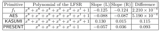
C: Slope of the linear complexity distribution

Here we present the results of the test in Section 5.2 in Table 5. The slope in Table 5 is the average slope over 108 _{samples. The column “Slope (L)” contains the slopes computed} from the LFSR input, and the column “Slope (R)” contains the slopes computed from the random input. The last column shows the absolute value of the difference between “Slope(L)” and “Slope(R)”. We can see the “Difference” of KASUMI and PRESENT are much greater than f1 and AES.

Table 5: The slope off1, AES, KASUMI and PRESENT on average

Primitive Polynomial of the LFSR Slope (L) Slope (R)|Difference|

f1 x8+x6+x4+x3+x2+x1+ 1 −0.125 −0.124 2.210×10−4

AES x8₊_x7₊_x6₊_x3₊_x2₊_x1_{+ 1} ₋_0.088 ₋_0.087 _5.190_×₁₀−4

KASUMI x8₊_x7₊_x6₊_x5₊_x4₊_x2_{+ 1} _0.130 _0.015 _0.115