Razvan Barbulescu, J´er´emie Detrey, Nicolas Estibals, and Paul Zimmermann
CARAMEL project-team, LORIA, Universit´e de Lorraine / INRIA / CNRS, Campus Scientifique, BP 239, 54506 Vandœuvre-l`es-Nancy Cedex, France
Abstract. We describe a unified framework to search for optimal formulae evaluating bi-linear — or quadratic — maps. This framework applies to polynomial multiplication and squaring, finite field arithmetic, matrix multiplication, etc. We then propose a new algorithm to solve problems in this unified framework. With an implementation of this algorithm, we prove the optimality of various published upper bounds, and find improved upper bounds.
Keywords: optimal algorithms, polynomial multiplication and squaring, finite field arith-metic, tensor rank, bilinear map, bilinear rank
1 Introduction
This article studies the bilinear rank problem. Given a field K, this problem naturally arises when considering the computational complexity of formulae (or algorithms) for evaluating bilinear maps over K [4, Ch. 14]. For instance, typical bilinear maps include — but are not limited to — the multiplication of twon-term polynomials ofK[X], or of two r×r square matrices ofKr×r.
Note that, given an algorithm for computing a bilinear map over K, this algorithm can be naturally extended to compute the same bilinear map over any larger K-algebra K. For instance, given a formula for computing the product of two n-term polynomials over K = F2, the exact same formula can also be used to compute the product of two
n-term polynomials over any field extensionK=F2m, or even the product of twon-term polynomials of Fr2×r[X], i.e., polynomials having binary r×r matrices as coefficients. A
nice illustration of the latter is given by Albrecht in [1], where the multiplication of large r×rmatrices overF2n is implemented by representingFr×r
2n asFr2×r[X]/hf(X)·Fr2×r[X]i, withf an irreducible polynomial overF2of degreen, and then using Montgomery’sn-term
polynomial multiplication formulae [16].
Therefore, when dealing with such formulae, a crucial distinction is made between
– afull multiplication a·bof two elementsaandbderived from the inputs of the bilinear map, and thus possibly living in the larger algebra K; and
– an addition a+b or a scalar multiplication λa, where λis given by the bilinear map only, and thus belongs to the smaller coefficient fieldK.
Intuitively, the first one is expected to have a much higher computational cost than the last two. Table 3 in [1] shows that the time needed to multiply two matrices over fields of characteristic 2 is proportional to the number of full multiplications in the formulae used for this purpose. A sensible way to optimize the overall complexity of the formula at hand is therefore to minimize the number of these full multiplications, which corresponds to solving a particular instance of the bilinear rank problem.
Definition of the problem. Let K be a field. Given an n ×m bilinear map φ : Kn×Km → K`, the bilinear rank problem consists in finding formulae for evaluat-ingφ involving a minimal number k of full multiplications. This optimalk is called the
bilinear rank of the mapφ.
More formally, considerB(Kn, Km;K) the set ofn×mbilinear formsfromKn×Kmto
K. Each such bilinear formγ can be written asγ :a,b7→P
i,jγi,jaibj, with the two input
vectors a = (a0, a1, . . . , an−1) ∈ Kn, b = (b0, b1, . . . , bm−1) ∈ Km, and the coefficients
γi,j ∈K. As γ is uniquely determined by the γi,j’s, we can represent B(Kn, Km;K) as
the vector space of dimension nm over K, which we will denote by V in the following. The representation of the bilinear form γ in V is therefore the nm-dimensional vector γ = (γ0,0, γ0,1, . . . , γn−1,m−1), and a bilinear map φ from Kn×Km to K` can then be
represented as a tuple of`vectors ofV:φ= (φ0, φ1, . . . , φ`−1)∈V`.
Consider now an n×m bilinear form γ. We say that γ is of rank 1 if there exist two linear forms α : Kn → K,a 7→ P
iαiai and β : Km → K,b 7→ Pjβjbj such that
γ(a,b) =α(a)·β(b) for alla∈Kn and b∈Km.
Rank-1 bilinear forms are particularly relevant in the context of the bilinear rank problem: indeed, each such form can be evaluated using only one full multiplication, as evaluating the two linear forms α and β at a and b, respectively, only requires scalar multiplications and additions. Furthermore, since the mapsei,j :a,b7→aibj are all
rank-1 bilinear forms, any bilinear form can then be written as a linear combination of rank-rank-1 bilinear forms:γ =P
i,jγi,jei,j. Therefore, one can ask the question: What is the minimal
number of rank-1 bilinear forms necessary to evaluate a given bilinear form? A given bilinear map?
In the case of a (single) bilinear formγ, the answer is easy: the bilinear rank is given by the actual rank of then×m matrix (γi,j)0≤i<n,0≤j<m formed by the coefficients ofγ.
However, the minimal number of full multiplications is much more difficult to compute when evaluating ` ≥ 2 bilinear forms simultaneously, such as is the case with bilinear maps: this is the aforementionedbilinear rank problem, formalized below.
Definition 1 (Bilinear rank problem [4, Ch. 14]). Using the above notations, and given a finite generator set G ⊂V composed of rank-1 n×m bilinear forms, along with a finite target set of ` bilinear forms T = {t0, t1, . . . , t`−1} ⊆ Span(G), the bilinear
rank problem consists in generating all the elements of T by K-linear combinations of a minimal number k of elements of G or, alternatively, to find all solutions for that optimal k.
Without loss of generality, the target vectors ti can further be assumed to be linearly
independent, as reconstructing an extra target vector by linear combination would only require scalar multiplications and additions.
Note that this problem can be adapted to also encompass the case of sets ofquadratic
forms. Indeed, any quadratic formσfromKntoK,σ :a7→P
0≤i≤j<nσi,jaiaj, is uniquely
represented by its coefficients σi,j ∈K. The set of n-ary quadratic forms Q(Kn;K) can
thus be seen as a vector space of dimensionn(n+1)/2 overK. It suffices then to takeV to be this vector space, and to define the rank-1 quadratic forms to be the quadratic forms σ for which there exist two linear forms overKn,α:a7→P
iαiai and α0 :a7→Piα0iai,
such thatσ(a) =α(a)·α0(a) for all a∈Kn.
In fact, anyn×mbilinear form can be seen as an (n+m)-ary quadratic form σ such that no product aiaj occurs between the first n or between the last m input variables:
σi,j = 0 for all 0≤i≤j < nand for all n≤i≤j < n+m. Hence, computing the rank
Also, the bilinear rank problem is NP-hard. Indeed, B¨urgisser et al. show in [4, Sec. 14.2] its equivalence to the decomposition of an order-3 tensor, known to be NP-hard [14].
Notation. Note that in the rest of this document, by an abuse of notation, we will omit writing the input vectors of the considered bilinear or quadratic forms, as they will always bea,bora, respectively. Hence, we will simply writeγ =P
i,jγi,jaibjorσ =Pi≤jσi,jaiaj
to refer to the corresponding forms in the following. This amounts to implicitly considering theai’s andbj’s as formal variables over K.
Related results. Several authors have considered special instances of the bilinear rank problem. We do not claim an exhaustive state-of-the-art here, but we mention the main results related to our work.
For polynomial multiplication, evaluation–interpolation algorithms like Karatsuba’s and Toom’s algorithms [15,20] are special cases of the problem, where the only full mul-tiplications involved correspond to evaluations of the product of the two polynomials at different points.
Even though the bilinear rank problem was already well known in the algebraic com-plexity community [4], until only recently, all the formulae used in the computer arith-metic community were based on this evaluation–interpolation scheme. In [16], instead of using only the evaluation products, i.e., (P
iκiai)(Pjκjbj) for some κ ∈ K,
Mont-gomery considered other rank-1 bilinear forms. This allowed him to find formulae with less products for the 5-, 6-, and 7-term polynomial multiplications, which do not fit in any evaluation–interpolation scheme. Montgomery however restricted the exploration to the set of “symmetric” generators of the form (P
iαiai)(Pjαjbj). Our work shows how
to improve Montgomery’s exploration and proves that the formulae in [16] are optimal for the 5-term polynomial multiplication.
In [9], Chung and Hasan propose asymmetric squaring formulae over Q, found using an exhaustive search method similar to that of Montgomery, but starting from an ad-hoc set of rank-1 generators. In [12], Fan and Hasan use Montgomery’s formulae and the Chinese Remainder Theorem together with a short product for the high degree terms to improve the bounds overF2; those results were further improved by Cenk and ¨Ozbudak
[5]. In [18], using both exhaustive and heuristic search algorithms, Oseledets considers the multiplication of n-term polynomials, and also their product modulo Xn — which corresponds to Mulders’ short product [17] — and modulo Xn+ 1. Some of the linear algebra routines he proposed are a building block in our method.
Multiplication in finite field extensions Fqn forn≥2 reduces to polynomial multipli-cation modulo a degree-nirreducible polynomialf overFq. Thus, one could first compute
a full product of twon-term polynomials, then reduce it modulof using only scalar mul-tiplications; however it is sometimes faster to directly compute thenterms of the product modulof [7].
Fast matrix multiplication is another application of the bilinear rank problem, with the smallest unsolved problem being the multiplication of two 3×3 matrices (for two square matrices): we know that at least 19 products are needed, and that 23 are enough, but the minimal rank is still unknown [3,11].
why it is pertinent to the computer algebra and computer arithmetic communities. Fol-lowing Montgomery [16], we see this problem in the light of linear algebra, which enables one to search for optimal formulae for a large set of applications such as polynomial mul-tiplication or squaring, matrix mulmul-tiplication, etc. Second, we propose a new algorithm to solve the bilinear rank problem; this algorithm is faster than Montgomery’s exploration algorithm [16] and is an improvement on Oseledets’ heuristic Minbas [18], which might
not find the minimal rank. Last, using this new algorithm we prove the optimality of several known formulae, and exhibit new bounds for some bilinear maps.
Roadmap. The article is organized as follows. After detailing a few instances of the bi-linear rank problem in Section 2, we show in Section 3 how this problem can be translated into a linear algebra problem. Section 4 gives an efficient algorithm solving this linear al-gebra problem. Finally Section 5 presents experimental results proving that some bounds from the literature are optimal, along with an improved bound for the multiplication in F35.
2 Some Instances of the Bilinear Rank Problem
Throughout the rest of this paper, we will use the following running example:
Example 1 (2 ×3-term polynomial product). We want to multiply A = a1X +a0 by
B = b2X2+b1X +b0 in K[X]. The naive algorithm requires 6 products, while only 5
products are necessary when using Karatsuba’s trick:
A·B =g3X3+ (g1+g2)X2+ (g4−g2−g0)X+g0,
whereg0=a0b0,g1 =a0b2,g2 =a1b1,g3=a1b2, andg4= (a0+a1)(b0+b1). Since A·B
has 4 terms, if the base field K contains at least 3 elements, evaluating A·B at those elements and at infinity —i.e., the a1b2 product — enables to recoverA·B by Lagrange
interpolation. However, ifK =F2, are 5 products optimal?
To illustrate the generality of the proposed framework, we give a few more examples:
Example 2 (3-term polynomial squaring [9]). We want to square the polynomial A = a2X2+a1X+a0 ∈K[X]. For this quadratic map, we have n = 3, the generator set G
consists of the 28 products
a20,a0a1,a0a2,a0(a0+a1), a0(a0+a2), a0(a1+a2), a0(a0+a1+a2),
a21,a1a2,a1(a0+a1),a1(a0+a2),a1(a1+a2),a1(a0+a1+a2),
a22,a2(a0+a1), a2(a0+a2), a2(a1+a2), a2(a0+a1+a2),
(a0+a1)2, (a0+a1)(a0+a2), (a0+a1)(a1+a2), (a0+a1)(a0+a1+a2),
(a0+a2)2, (a0+a2)(a1+a2), (a0+a2)(a0+a1+a2),
(a1+a2)2, (a1+a2)(a0+a1+a2),
(a0+a1+a2)2,
and the target set is
T ={t0:=a20, t1 := 2a0a1, t2 :=a21+ 2a0a2, t3:= 2a1a2, t4 :=a22},
Example 3 (Middle product [13]). Assume we only want to compute the degree-1 and -2 coefficients of the productA·B from Example 1. We haven= 2,m= 3, and Gis the set of all rank-1 bilinear forms of the form (α0a0+α1a1)(β0b0+β1b1+β2b2) for αi, βj ∈K.
The target set is
T ={t0 :=a0b1+a1b0, t1 :=a0b2+a1b1}.
A solution with k= 3 considers the subset
{g0 :=a0(b1+b2), g1 :=a1(b0+b1), g2:= (a1−a0)b1} ⊆ G,
which gives the formulaet0 =g1−g2 and t1=g0+g2.
Example 4 (3×3 matrix multiplication).Here, n=m = 9, and we consider the product A·B overK3×3 of the two matrices
A=
a0 a1 a2
a3 a4 a5
a6 a7 a8
and B=
b0b1 b2
b3b4 b5
b6b7 b8 .
The target setT consists of the 9 bilinear forms{a0b0+a1b3+a2b6, ..., a6b2+a7b5+a8b8},
and the generator set G consists of the non-zero rank-1 bilinear forms (α0a0 +· · · +
α8a8)(β0b0+· · ·+β8b8) for αi, βj ∈K,i.e., (29−1)2 = 261 121 forms forK =F2.
3 From Bilinear Applications to Linear Algebra
We focus in the rest of the paper on bilinear maps, the case of quadratic maps being similar. Recall that we denote byV the vector space of dimensionnmoverK isomorphic to the space ofn×mbilinear forms B(Kn, Km;K). Thus, each element of T and G (see
Definition 1) being such a bilinear form, it can be written as a row vector of dimension nm, where the (im+j)-th column corresponds to the coefficient of the aibj term.
Example 1 (Cont’d).For our running example of the 2×3-term polynomial multiplication overK =F2, the canonical basis of the vector spaceV is (a0b0, a0b1, a0b2, a1b0, a1b1, a1b2).
The target set is T ={a0b0, a0b1+a1b0, a0b2+a1b1, a1b2}, and the set of generators G
consists of the 21 products:
G ={a0b0, a1b0, (a0+a1)b0,
a0b1, a1b1, (a0+a1)b1,
a0(b0+b1), a1(b0+b1), (a0+a1)(b0+b1),
a0b2, a1b2, (a0+a1)b2,
a0(b0+b2), a1(b0+b2), (a0+a1)(b0+b2),
a0(b1+b2), a1(b1+b2), (a0+a1)(b1+b2),
a0(b0+b1+b2), a1(b0+b1+b2), (a0+a1)(b0+b1+b2) }.
We can then rewriteT as the following matrix of 4 row vectors:
T =
a0b0a0b1a0b2a1b0a1b1a1b2
1 0 0 0 0 0
0 1 0 1 0 0
0 0 1 0 1 0
0 0 0 0 0 1
a0b0
a0b1+a1b0
a0b2+a1b1
The same applies to the set of generators G, which gives the 21×6 matrix:
G=
a0b0a0b1a0b2a1b0a1b1a1b2
1 0 0 0 0 0
0 0 0 1 0 0
1 0 0 1 0 0
..
. ... ... ... ... ...
1 1 1 1 1 1
a0b0
a1b0
(a0+a1)b0
.. .
(a0+a1)(b0+b1+b2)
The bilinear rank problem is then stated as follows: For a given integerk, we want to find the subsetsW of k elements ofG such that the subspace W spanned by W contains T. In linear algebra terms, we want to find the subsets ofk rows of G whoseK-linear span contains all the row vectors ofT,i.e., contains the subspace T = Span(T).
4 Solving the Linear Algebra Problem
We recall the notations from Definition 1:V is the vector space of dimensionnmspanned by the aibj products, G ⊂ V is a finite set of generators, T ⊆ Span(G) is the set of
target vectors, andT = Span(T) is the corresponding target space spanned by the target vectors, which has dimension`.
In the previous section, we reduced our problem of finding all formulae with k full multiplications for evaluating a given bilinear map to a linear algebra problem: given a finite subsetGof a K-vector spaceV and a target subspaceT = Span(T) of Span(G), we want to find all the rank-k subspaces W of V containing T and which can be generated by elements ofG only (i.e., Span(W ∩ G) =W). One should note that this linear algebra problem is more general than the original problem of optimizing the computation of bilinear maps.
4.1 Naive Algorithm
A trivial approach to the linear algebra problem is to enumerate all the #kG subsets W ={g1, . . . , gk} ofG and, for each of them, test if its span covers T. The most efficient
way to test this inclusion of spaces is to constructW = Span(W), represented by its basis as a matrix in row echelon form, and then test if each vector t∈ T reduces to 0 against this matrix.
For simplicity’s sake, in this paper we focus on the combinatorial complexity of the algorithms, considering that all matrix operations (e.g., computing the dimension of a vector space, checking if a vector is in a vector space, computing the row-echelon form of a matrix) have constant complexity. The complexity of the naive algorithm is thus
#G k
.
Example 1 (Cont’d). For the 2×3-term polynomial multiplication, #G= 21, k= 5. We therefore have to test 20 349 subsetsW.
4.2 Improved Algorithm
The main drawback of the naive algorithm is that different subsets of generatorsWi may
the multiplication of two 3-term polynomials overQ, Montgomery [16] gives the following family of solutions:
(a0+a1X+a2X2)(b0+b1X+b2X2) =a0b0(C+ 1−X−X2) (1)
+a1b1(C−X+X2−X3) +a2b2(C−X2−X3+X4)
+(a0+a1)(b0+b1)(−C+X) + (a0+a2)(b0+b2)(−C+X2)
+(a1+a2)(b1+b2)(−C+X3) + (a0+a1+a2)(b0+b1+b2)C.
Taking different values for the arbitrary polynomialC ∈Q[X], we see that any subset of 6 out of the 7 generatorsG={a0b0, a1b1, a2b2,(a0+a1)(b0+b1),(a0+a2)(b0+b2),(a1+
a2)(b1 +b2),(a0 +a1+a2)(b0 +b1 +b2)} yields a solution. However, these 7 solutions
correspond to the same vector spaceW, since the 7 generators are linearly dependent:
(a0+a1+a2)(b0+b1+b2) = (a0+a1)(b0+b1) + (a0+a2)(b0+b2)
+ (a1+a2)(b1+b2)−a0b0−a1b1−a2b2.
We propose an algorithm that takes advantage of this redundancy by looking directly for the subspacesW — instead of the subsets of generators — that cover our target space T. More formally, we search all the subspaces W of V such that:
(i) T ⊂W,i.e., the target spaceT is covered by W;
(ii) Span(W ∩ G) =W,i.e.,W is spanned by elements of G; and (iii) dimW =k,i.e., only k generators are needed.
A first remark is that from (i), the target spaceT is contained in each solution space W. Thus we should look for all the W’s by extending this vector space. Unfortunately, there are a lot of spaces aboveT, possibly more than there are subsets W of G. Instead, we might consider only those spaces W which are obtained by adding generators to T. This technique has already been used by Oseledets [18] in some heuristic algorithms. In order to use this idea without losing the exhaustiveness of our algorithm, we introduce a new condition:
(ii0) ∃W0 ⊂ G such thatW =T⊕Span(W0).
Lemma 1. All subspaces W that verify (i) and (ii) also verify (ii0).
Proof. Let W a subspace verifying (i) and (ii), the result follows directly from Proposi-tion 1 withH beingW ∩ G, and F being the free family T ⊂W. ut
Proposition 1 ([2, Prop. 3.15]). Let W be a vector space over a field K spanned by a finite set of generators H. Let F be a free family of W. Then there exists a subset J of
Hsuch that F ∪ J is a basis of W.
Proof. IfF generates W then we take J =∅.
Algorithm 1Find all the subspaces of dimensionkgenerated by elements ofG only and that contain the target spaceT.
Input: A vector spaceV, a finite setG of elements ofV, a subspaceT ofV included in Span(G), and an integerksuch that dimT≤k≤rk(G).
Output: The setS of all subspacesW ofV such thatT ⊂W, Span(W∩ G) =W, and dimW =k. 1. S ← ∅
2. procedureexpand subspace(W)
3. ifdimW =kandrk(W ∩ G) =kthen 4. S ← S ∪ {W}
5. else ifdimW < kthen 6. for eachg∈ G \W do
7. expand subspace(W ⊕Span(g)) 8. end procedure
9. expand subspace(T) 10. return S
Thanks to Lemma 1, finding all subspacesW of V verifying conditions (i), (ii), and (iii) can be achieved by first enumerating all subsetsW0ofGsuch thatW =T⊕Span(W0) verifies conditions (i), (ii0), and (iii), and then keeping only those for whichW also verifies condition (ii). This method is implemented in Algorithm 1, which is proven correct in Theorem 1.
Theorem 1 (Correctness of Algorithm 1). For any given k, Algorithm 1 returns all the subspaces W of V verifying conditions (i), (ii) and (iii). In particular, when Algorithm 1 fails to find any solutions for allk under a boundk0, then no solutions exist below this bound, and the bilinear rank is greater or equal to k0.
Proof. Let W be a subspace of V verifying (i), (ii) and (iii). We first prove that W is included in the output of Algorithm 1. By Lemma 1,W also satisfies (ii0). Thus there is a subset W0 ={g1, ..., gk0} of G such that W =T ⊕Span(g1, ..., gk0), and we can choose g1, ..., gk0 to be linearly independent. Therefore, Algorithm 1 will, at some point in the enumeration, consider the candidate subspaceW. Since dimW =kand, by condition (ii) we have rk(W ∩ G) = dimW =k, Algorithm 1 will include W inS.
Conversely, let W in the output of Algorithm 1; let us show that conditions (i), (ii), and (iii) are fulfilled. Condition (i) is trivially verified, since Algorithm 1 constructsW by expanding the initial subspaceT. Furthermore, sinceW is inS, we have dimW =k, thus (iii) is also verified. Finally, we have rk(W ∩ G) =k, which implies Span(W ∩ G) =W,
and thusW also fulfills condition (ii). ut
Example 1 (Cont’d). For our running example, Algorithm 1 immediately shows that no solutions exist withk = 4 over F2. Indeed, we have dimT = 4, thus dimW = 4 at the
very first call ofexpand subspace, but the rank of W ∩ G is only 3.
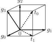
Example 5 (Step-by-step illustration of Algorithm 1).Take K=Q,V =Q3,T ={t0, t1}
with t0 = (1,1,1) and t1 = (1,1,0); and G = {g0, g1, g2, g3} with g0 = (1,0,0), g1 =
(0,1,0),g2= (0,0,1), andg3 = (1,0,1), as depicted in Figure 1. In this example, for
clar-ity’s sake, we denote the recursive depth of the current call by a parenthesized superscript:
e.g.,W(i) represents the subspaceW at recursive depthi, starting ati= 0.
Let us first consider the casek= 2. The algorithm initializesW(0) toT = Span(t0, t1),
which is already of dimension 2. It then computes W ∩ G = {g2}, which is of rank 1.
Therefore, there are no solutions fork= 2.
Fig. 1.The setsG andT from Example 5.
g0 g3
g1
t1 g2
t0
0
G \W(0) ={g0, g1, g3}. Takingg=g0 and adding it toW(0), the algorithm recurses down
withW(1)=T⊕Span(g0). We haveW(1)∩ G ={g0, g1, g2, g3}, which has rank 3, meaning
that this W(1) is a solution subspace, which is then added to the set S. The algorithm can now reiterate the process for the subspaces W(0)⊕Span(g1) and W(0) ⊕Span(g3),
finding both of them to also be solutions.
Note that there is no point to try the algorithm for k > 3: since dimV = 3, the algorithm will never find subspacesW ofV of dimensionk.
Remark also that this simple example illustratesrank leapsforW∩G: if rk(W(0)∩G) =
1, when taking W(1) = W(0) ⊕Span(g0), the rank of W(1) ∩ G jumps directly to 3. In
fact, since T cannot usually be generated by elements of G only, we have dimW(0) > rk(W(0)∩G) at the beginning of the algorithm. Therefore, since dimW is only incremented by 1 at each recursive call, rank leaps between W(i)∩ G and W(i+1)∩ G gradually close the gap between dimW and rk(W ∩ G).
Example 6 (Evaluation–interpolation schemes).In the case of then-term polynomial mul-tiplication over a fieldK, evaluating the resulting polynomial at a point κ ∈K only in-volves a linear combination of the target coefficientsti. Therefore, the rank-1 bilinear forms
(P
iκiai)(
P
jκjbj) corresponding to the evaluation of the two input polynomials atκare
also inT. This is also the case when evaluating “at infinity”,i.e., considering the leading coefficientan−1bn−1. Therefore, since these rank-1 bilinear forms are linearly independent
(by Vandermonde determinant), if #K ≥2n−2, then we have rk(T ∩ G) = 2n−1 =`, andT itself is a solution subspace.
4.3 Implementation Issues
Algorithm 1 relies extensively on operations on vector spaces, such as computing the rank of the intersection W ∩ G (line 3), or excluding elements of W from G (line 6). In order to perform these operations efficiently, each subspaceW is represented in the algorithm by the r×nm matrix of its basis in row echelon form, where r = dimW. Note that we also denote byW the matrix in row echelon form corresponding to the subspaceW.
Computing WG = Span(W ∩ G) is done as follows: first reduce every vector g∈ G by the matrixW; ifg reduces to the null vector, then g∈W. For each such g, reduce it by the current matrixWG (initially empty), and if the reduced vector is not null, add it to WG. OnceWG is constructed, the rank ofW ∩ G is then given by the number of rows of the matrix.
are identical, and recursing down the algorithm for both of them would just be a waste of time. Maintaining a setH of reduced generators prevents this to happen, asg and g0 will then correspond to a single reduced generator inH. Furthermore, at recursion depth i, since all elements g ofH(i) are reduced byW(i), when recursing down the algorithm:
– constructing W(i+1) = W(i)⊕Span(g) only requires inserting the row vector g into the matrixW(i); and
– reducing each elementh ∈ H(i) by W(i+1) to construct H(i+1) only requires reducing
h by Span(g), as it is already reduced by W(i).
Example 1 (Cont’d).On our running example,T = Span(T) is the 4×6 matrix — which is already in row echelon form — andG consists of the 21 generators from Section 3. Let us follow the execution of the algorithm in the case k= 5.
We first constructH(0) by reducing all generators of G by W(0) =T. Only 3 unique
reduced generators remain:
H(0)=
a0b0a0b1a0b2a1b0a1b1a1b2
0 0 0 1 0 0
0 0 0 0 1 0
0 0 0 1 1 0
a1b0
a1b1
a1(b0+b1)
Since dimW(0) = 4< k, these generators inH(0)are then enumerated, and the procedure
expand subspace is called recursively for each of them.
For instance, when taking g= a1b0, the subspace W(1) is constructed by inserting g
into the matrixW(0):
W(1) =
a0b0 a0b1 a0b2 a1b0 a1b1a1b2
1 0 0 0 0 0
0 1 0 1 0 0
0 0 1 0 1 0
0 0 0 1 0 0
0 0 0 0 0 1
a0b0
a0b1+a1b0
a0b2+a1b1
g=a1b0
a1b2
Computing W(1)∩ G yields a set of 9 generators and of rank 5; W(1) is thus a solution
subspace.
Finally, continuing the enumeration for g=a1b1 theng =a1(b0+b1), the algorithm
will find two other solution subspaces of rank 5.
4.4 From Solution Subspaces back to Formulae
Given a solution subspace W verifying conditions (i), (ii), and (iii), we still need to retrieve the corresponding formulae. Note that since T ⊂ W, each formula corresponds to a basis ofW using only generators fromG. A simple solution is thus to first compute the setW ∩ G, then enumerate all subsets of klinearly independent vectors inW ∩ G.
For every basis ofW, obtaining the corresponding formula is then just a matter of find-ing the coordinates of the vectors ofT in this basis, which will give us the corresponding linear combinations of generators required to compute them.
4.5 Complexity Analysis
Algorithm 1 allows us to drastically reduce the number of operations required to find all the formulae for evaluating a given bilinear map thanks to the two following key ideas:
1. searching for subspacesW of Span(G) instead of subsetsW of G; and 2. constructing these subspaces starting fromT instead of{0}.
The algorithm consists in expanding T to a vector space of dimension k by adding k−`vectors fromG, where`= dimT. The combinatorial complexity of the algorithm is thus bounded by:
#G k−`
.
Note however that this complexity bound does not reflect the gain due to the first idea — searching for subspaces instead of subsets — since that gain depends on the particular problem to be solved, and cannot be expressed simply. In Algorithm 1, once sayg1, g2, . . . have been added to the initialW(0)=T, this idea will prune the remaining
set of independent generatorsG \W (without this idea, instead of considering allg∈ G \W at line 6 of Algorithm 1, we would consider allg∈ G, which would be very similar to the naive algorithm). Note however that Algorithm 1 does not guarantee that all subspaces W explored and found to be solutions are different. Duplicates have to be detected and removed upon adding solution subspaces to the setS.
In practice, this combinatorial complexity is usually not attained, as can be seen in the experimental results reported in Section 5.
Example 1 (Cont’d).For the 2×3-term polynomial multiplication overF2, with #G= 21, k= 5, and `= 4, the complexity estimate predicts 21 subspacesW to consider, whereas in practice, only 3 of these subspaces need be explored by the algorithm. This has to be compared with the 20 349 subsets explored by the naive algorithm.
4.6 Special Case of Symmetric Bilinear Maps
An n×n bilinear form γ :a,b 7→ P
i,jγi,jaibj is said to be symmetric if γi,j =γj,i for
all 0≤i, j < n. Similarly, an n×nbilinear mapφ is said to besymmetric if the bilinear forms corresponding to its coefficients are all symmetric. For instance, it is the case for then-term polynomial multiplication.
Example 7 (3-term polynomial multiplication). Given A = a2X2+a1X +a0 and B =
b2X2+b1X+b0∈K[X], the target set for the productA·B is
T ={a0b0, a0b1+a1b0, a0b2+a1b1+a2b0, a1b2+a2b1, a2b2},
all of whose bilinear forms are symmetric.
In the case where the target set T is composed only of symmetric forms, an idea to accelerate the search for formulae is to restrictGto be the set of rank-1 symmetric bilinear forms, which are of the form (P
iαiai)(Pjαjbj). Indeed, while there are (#K)n
2
−1 non-zero bilinear forms of rank 1 in B(Kn, Kn;K), only (#K)n−1 of them are symmetric,
which yields a huge speedup.
However, the symmetric rank-1 forms alone may fail to produce optimal formulae for symmetric maps: for instance,a0b1+a1b0cannot be computed with 2 symmetric products
over F2. (For an introduction on the topic of decomposing symmetric maps as sums of
5 Experimental Results
We present here some results obtained for various instances of the bilinear rank problem using a multi-threaded C implementation of Algorithm 1. The reported timings correspond to the total execution time on a single core of a 2.2 GHz Xeon L5640. We reproduce or improve some known results [7,9,16] but also find the complete list of solutions for each problem or prove lower bounds thanks to Theorem 1.
In all the following tables, only one value forkis reported for each problem. It is the smallest possible value for which solutions were found or, if no solutions were found, it is the largest value which was tried with our algorithm. In both cases, it means that there are no solutions for smaller values of k. Rows without a value for k were deemed too computationally expensive and were not tried at all with our implementation.
Under the heading “# of tests” are reported the number of subspacesW for which the algorithm had to check whether rk(W ∩ G) =k or not. It corresponds to the number of leaves in the tree of recursive calls. The column “# of solutions” reports the number #S of solution subspaces returned by Algorithm 1. Finally, we indicate in the column “# of formulae” the corresponding number of formulae, or∞when this number is really large. Finally, where applicable and when an exhaustive search using all rank-1 bilinear forms forG was too expensive, we enumerated subspaces using only symmetric generators. This is indicated by a “(Sym.)” mention next to the cardinality ofG.
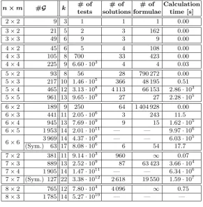
Thus, Table 1 gives experimental results for n×m-term polynomial multiplication overF2. For instance, the 6×6 row indicates that there are no formulae with onlyk= 14
full multiplications overF2; however, symmetric formulae exist fork= 17. Similarly, the
5×5 row shows that Montgomery’s bound ofk= 13 is optimal overF2 [16]. Table 2 gives
similar results overF3. For example, the 5×5 row with no solution fork= 11 proves that
the boundM3(5) = 12 from [6, Table 2] is optimal.
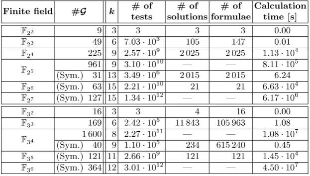
Table 3 corresponds to small extensions ofF2orF3, where we consider the
multiplica-tion of two elements in polynomial basis. This is relevant for example for multiplicamultiplica-tion of matrices overF2e [1]. In particular the rowsF24 withk= 9 andF34 withk= 6 confirm
the values from [7, Table 1].
Furthermore, according to the literature, the best known formula for computing the product of two elements over the finite fieldF35 uses 12 full multiplications [7]. As indicated
in Table 3, our algorithm found 121 symmetric formulae using only 11 full multiplications. One such formula is given in Algorithm 2.
Finally, Table 4 considers the product of two n-term polynomials modulo Xn and Xn−1 over F2 — as in [18] — and also over F3. This proves the tensor rank from [18]
is the optimal one forn= 2,3,4 over F2 modulo both Xn and Xn−1. One should note
that overF3, computing a product moduloX4−1 can be done with the same number of
products (5) than moduloX3−1.
6 Conclusion
Table 1.Experimental results forn×mpolynomial multiplication overF2.
n×m #G k # of # of # of Calculation
tests solutions formulae time [s]
2×2 9 3 1 1 1 0.00
3×2 21 5 2 3 162 0.00
3×3 49 6 9 3 9 0.00
4×2 45 6 5 4 108 0.00
4×3 105 8 700 33 423 0.00
4×4 225 9 6.60·103 4 4 0.03 5×2 93 8 56 28 790 272 0.00 5×3 217 10 1.46·105 366 48 195 0.51 5×4 465 12 3.13·108 4 113 66 153 2.86·103 5×5 961 13 9.65·109 27 27 2.28·105 6×2 189 9 250 64 1 404 928 0.00 6×3 441 11 2.05·106 3 243 11.5 6×4 945 13 7.69·109 9 15 1.62·105 6×5 1 953 14 2.01·1011 — — 9.97·106 6×6 3 969 14 4.37·10
9
— — 6.03·105 (Sym.) 63 17 8.08·106 6 54 17.7 7×2 381 11 9.14·103 960 ∞ 0.07 7×3 889 13 2.52·109 87 63 423 3.66·104 7×4 1 905 14 1.47·1011 — — 6.34·106 7×7 (Sym.) 127 22 3.38·1012 2 618 19 550 1.59·107 8×2 765 12 7.80·104 4 096 ∞ 0.75 8×3 1 785 14 5.27·1010 — — —
Table 2.Experimental results forn×mpolynomial multiplication overF3.
n×m #G k # of # of # of Calculation
tests solutions formulae time [s]
2×2 16 3 1 1 4 0.00
3×2 52 4 1 1 1 0.00
3×3 169 6 24 22 1 493 0.00 4×2 160 6 9 13 38 880 0.00
4×3 520 7 164 12 48 0.00
4×4 1 600 9 4.11·105 726 50 640 14.9 5×2 484 7 24 36 93 312 0.00 5×3 1 573 9 2.81·105 1 116 94 629 9.33 5×4 4 840 10 4.75·106 48 768 1.01·103 5×5 14 641 11 4.89·10
7
Table 3.Experimental results for multiplication over small extensions ofF2andF3.
Finite field #G k # of # of # of Calculation
tests solutions formulae time [s]
F22 9 3 3 3 3 0.00
F23 49 6 7.03·103 105 147 0.01
F24 225 9 2.57·109 2 025 2 025 1.13·104
F25
961 9 3.10·1010 — — 8.11·105 (Sym.) 31 13 3.49·106 2 015 2 015 6.24 F26 (Sym.) 63 15 2.21·1010 21 21 6.63·104
F27 (Sym.) 127 15 1.34·1012 — — 6.17·106
F32 16 3 3 4 16 0.00
F33 169 6 2.42·105 11 843 105 963 1.08
F34 1 600 8 2.27·10
11
— — 1.08·107 (Sym.) 40 9 1.10·105 234 615 240 0.45 F35 (Sym.) 121 11 2.66·109 121 121 1.45·104
F36 (Sym.) 364 12 3.01·1012 — — 4.50·107
Table 4. Experimental results for the multiplication of two n-term polynomials in Fp[X]/(Xn) and Fp[X]/(Xn−1), withp= 2 and 3.
Ring n #G k # of # of # of Calculation
tests solutions formulae time [s]
F2[X]/(Xn)
2 9 3 3 3 10 0.00
3 49 5 590 12 40 0.00
4 225 8 5.17·107 1 440 9 248 230 5 961 9 2.66·10
10 — — 6.70·105 (Sym.) 31 11 3.64·105 112 736 0.48 6 (Sym.) 63 14 2.63·109 384 2 816 7.66·103 7 (Sym.) 127 15 1.16·1012 — — 5.46·106
F2[X]/(Xn−1)
2 9 3 3 3 10 0.00
3 49 4 21 3 3 0.00
4 225 8 2.69·107 1 440 9 248 124 5 961 9 1.39·10
10 — — 3.65·105 (Sym.) 31 10 7.46·104 25 25 0.09 6 (Sym.) 63 12 2.33·107 31 148 50.0 7 (Sym.) 127 13 2.55·109 1 49 1.24·104
F3[X]/(Xn)
2 16 3 4 4 39 0.00
3 169 5 7.94·103 90 1 539 0.07 4 1 600 7 5.54·10
8 — — 3.22·104 (Sym.) 40 8 3.17·105 252 40 095 0.14 5 (Sym.) 121 10 1.45·108 243 13 122 2.28·103 6 (Sym.) 364 11 4.79·1010 — — 8.22·105
F3[X]/(Xn−1)
2 16 2 1 1 1 0.00
3 169 5 4.45·103 90 1 539 0.04
4 1 600 5 767 4 16 0.07
Algorithm 2Multiplication over F35 ∼=F3[X]/(X5−X+ 1).
Input: A=a4X4+a3X3+a2X2+a1X+a0∈F35 andB=b4X4+b3X3+b2X2+b1X+b0∈F35.
Output: A·Bmod (X5−X+ 1) =t4X4+t3X3+t2X2+t1X+t0∈F35.
1. g0←a4b4 g5←(a0+a1−a2)(b0+b1−b2) 2. g1←(a0+a2)(b0+b2) g6←(a1−a3+a4)(b1−b3+b4) 3. g2←(a0−a3)(b0−b3) g7←(a2+a3−a4)(b2+b3−b4)
4. g3←(a1−a4)(b1−b4) g8←(a0+a1−a2−a3)(b0+b1−b2−b3) 5. g4←(a3−a4)(b3−b4) g9←(a0+a1−a3+a4)(b0+b1−b3+b4) 6. g10←(a1+a2−a3−a4)(b1+b2−b3−b4) 7. t0←g0+g2−g3−g4+g5+g6−g8
8. t1←g1+g2+g3+g4−g5−g8+g10 9. t2←g1−g2−g3−g5−g6−g7+g8 10. t3← −g0−g3+g4+g5−g7−g8+g10
11. t4← −g1+g2−g4+g5+g6+g7+g8+g9−g10 12. return t4X4+t3X3+t2X2+t1X+t0
overF2, in addition to the 7 possible formulae from Eq. (1) already found by Montgomery
in [16], we found two new asymmetric formulae, the first one using the generators
g1 :=a0b0, g2 :=a2b2, g3 := (a0+a1)(b0+b2), g4 := (a0+a2)(b1+b2),
g5 := (a1+a2)(b0+b1), g6:= (a0+a1+a2)(b0+b1+b2),
with (a0+a1X+a2X2)(b0+b1X+b2X2) being equal to:
g1+ (g2+g3+g5+g6)X+ (g3+g4+g6)X2+ (g1+g4+g5+g6)X3+g2X4,
and the second one using the generators
a0b0, a2b2,(a0+a1)(b1+b2),(a0+a2)(b0+b1),(a1+a2)(b0+b2),(a0+a1+a2)(b0+b1+b2).
It would be interesting to give a simple mathematical explanation for these new formulae. We were also able to improve the bound from [8] for the multiplication inF35 from 12
to 11 multiplications, using again a completely generic method.
If one wants to go further, one has to either speed up the computations or to use more heuristic or proven techniques borrowed to the algebraic complexity community: re-stricting the setGof products,e.g., to symmetric products for polynomial multiplication, enlarging the target setT by imposing that some products have to occur in the formula or using the symmetries of the problem.
Acknowledgements. The authors would like to thank Marc Mezzarobba for the inter-esting and fruitful discussions we had on the subject, especially for his knowledge of the many results on this topic.
References
1. Albrecht, M.R.: The M4RIE library for dense linear algebra over small fields with even characteristic. http://arxiv.org/abs/1111.6900(2011), preprint
2. Artin, M.: Algebra. Prentice-Hall, Inc. (1991)
3. Bl¨aser, M.: On the complexity of the multiplication of matrices of small formats. Journal of Complexity 19, 43–60 (2003)
4. B¨urgisser, P., Clausen, M., Shokrollahi, M.: Algebraic complexity theory, vol. 315. Springer Verlag (1997)
6. Cenk, M., ¨Ozbudak, F.: Efficient multiplication in F3`m,m ≥1 and 5 ≤` ≤18. In: Vaudenay, S.
(ed.) Proc. AFRICACRYPT 2008. Lecture Notes in Comput. Sci., vol. 5023, pp. 406–414 (2008) 7. Cenk, M., ¨Ozbudak, F.: On multiplication in finite fields. J. Complexity 26, 172–186 (2010)
8. Cenk, M., ¨Ozbudak, F.: Multiplication of polynomials moduloxn. Theoret. Comput. Sci. 412, 3451–
3462 (2011)
9. Chung, J., Hasan, M.A.: Asymmetric squaring formulae. In: Kornerup, P., Muller, J.M. (eds.) Proc. ARITH 18. pp. 113–122 (2007)
10. Comon, P., Golub, G., Lim, L., Mourrain, B.: Symmetric tensors and symmetric tensor rank. SIAM J. Matrix Anal. & Appl. 30(3), 1254–1279 (2008)
11. Courtois, N.T., Bard, G.V., Hulme, D.: A new general-purpose method to multiply 3×3 matrices using only 23 multiplications.http://arxiv.org/abs/1108.2830(2011), preprint
12. Fan, H., Hasan, A.: Comments on five, six, and seven-term Karatsuba-like formulae. IEEE Trans. Comput. 56(5), 716–717 (2007)
13. Hanrot, G., Quercia, M., Zimmermann, P.: The middle product algorithm, I. Speeding up the division and square root of power series. Appl. Algebra Engrg. Comm. Comput. 14(6), 415–438 (2004) 14. Hastad, J.: Tensor rank is NP-complete. J. Algorithms 11(4), 644–654 (1990)
15. Karatsuba, A.A., Ofman, Y.: Multiplication of multi-digit numbers on automata (in Russian). Doklady Akad. Nauk SSSR 145(2), 293–294 (1962), translation inSoviet Physics-Doklady 7, 595–596 (1963) 16. Montgomery, P.: Five, six, and seven-term Karatsuba-like formulae. IEEE Trans. Comput. 54(3),
362–369 (2005)
17. Mulders, T.: On short multiplications and divisions. Appl. Algebra Engrg. Comm. Comput. 11(1), 69–88 (2000)
18. Oseledets, I.: Optimal Karatsuba-like formulae for certain bilinear forms in GF(2). Linear Algebra and its Applications 429, 2052–2066 (2008)
19. Strassen, V.: Gaussian elimination is not optimal. Numerische Mathematik 13(4), 354–356 (1969) 20. Toom, A.: The complexity of a scheme of functional elements realizing the multiplication of integers.
In: Soviet Mathematics Doklady. vol. 3, pp. 714–716 (1963)
Appendix
We compare here Algorithm 1 to Oseledets’ work. The main similarity is that both meth-ods use a linear algebra setting and search for solution spacesW rather than solution sets W of generators. In terms of differences, we note that Algorithm 1 is proven, making it a tool for proving lower bounds (cf. Section 5). Oseledets’ work presents a main algorithm calledMinbas, a subroutine calledRank-1 and some more tricks.
Minbasstarts by computing the rank of all #KdimT−1 elements ofT (denotedC in
[18]), where the rank of a bilinear form is the minimalksuch that t=g1+g2+· · ·+gk
withgi ∈ G.Minbas continues by constructing a basis of T by adding in order linearly
independent elements of rank 1, 2 and so on. In our setting, the rank-1 elements from [18] are elements of the target space which are also in the set G of generators. Since Algorithm 1 starts by W =T, those forms are automatically included in our algorithm. From this point on, the two algorithms diverge since Algorithm 1 explores spaces W of higher dimension whereasMinbas adds forms of rank 2 or more.
The second algorithm of Oseledets’ work is called Rank-1 and can be used as a
subroutine in algorithms solving the bilinear rank problem. Given a candidate space W of dimension k lying above T, the Rank-1 procedure tests if W contains a basis made
out of elements inG by writing the lines of W and G in row echelon form. In our setting this is equivalent to the test rk(W ∩ G) =k.
written asW =T ⊕ hg1, ..., gk−dimTi. One recognizes the idea of replacing condition (ii)