Acquisition and Reconstruction Techniques for Fat Quantification Using Magnetic Resonance Imaging

(1)

Electronic Thesis and Dissertation Repository

11-25-2014 12:00 AM

Acquisition and Reconstruction Techniques for Fat Quantification

Using Magnetic Resonance Imaging

Abraam S. Soliman

The University of Western Ontario Supervisor

Charles A. McKenzie

The University of Western Ontario Joint Supervisor Terry M. Peters

The University of Western Ontario

Graduate Program in Biomedical Engineering

A thesis submitted in partial fulfillment of the requirements for the degree in Doctor of Philosophy

Follow this and additional works at: https://ir.lib.uwo.ca/etd

Part of the Biophysics Commons, and the Medical Biophysics Commons

Recommended Citation Recommended Citation

Soliman, Abraam S., "Acquisition and Reconstruction Techniques for Fat Quantification Using Magnetic Resonance Imaging" (2014). Electronic Thesis and Dissertation Repository. 2526.

https://ir.lib.uwo.ca/etd/2526

This Dissertation/Thesis is brought to you for free and open access by Scholarship@Western. It has been accepted for inclusion in Electronic Thesis and Dissertation Repository by an authorized administrator of

(2)

ACQUISITION AND RECONSTRUCTION TECHNIQUES

FOR FAT QUANTIFICATION USING MAGNETIC RESONANCE

IMAGING

(Thesis format: Integrated Article)

by

Abraam S. Soliman

Graduate Program in Biomedical Engineering

A thesis submitted in partial fulfillment

of the requirement for the degree of

Doctor of Philosophy

The School of Graduate and Postdoctoral Studies

The University of Western Ontario

London, Ontario, Canada

(3)

ii

Quantifying the tissue fat concentration is important for several diseases in various organs including liver, heart, skeletal muscle and kidney. Uniquely, MRI can separate the signal from water and fat in-vivo, rendering it the most suitable imaging modality for non-invasive fat quantification. Chemical-shift-encoded MRI is commonly used for quantitative fat measurement due to its unique ability to generate a separate image for water and fat. The tissue fat concentration can be consequently estimated from the two images. However, several confounding factors can hinder the water/fat separation process, leading to incorrect estimation of fat concentration.

The inhomogeneities of the main magnetic field represent the main obstacle to water/fat separation. Most existing techniques rely mainly on imposing spatial smoothness constraints to address this problem; however, these often fail to resolve large and abrupt variations in the magnetic field. A novel convex relaxation approach to water/fat separation is proposed. The technique is compared to existing methods, demonstrating its robustness to resolve abrupt magnetic field inhomogeneities.

(4)

iii

precise MRI fat quantification. Novel acquisitions and reconstruction techniques that address the current challenges for fat quantification are proposed.

(5)

iv

Chapter 2 is adapted from a published work in Springer Lecture Notes in Computer Sciences (LNCS) of Medical Image Computing and Computer-Assisted Intervention (MICCAI) 2012, entitled: “A Convex Relaxation Approach to Fat/Water Separation with Minimum Label Description” by Abraam Soliman, Jing Yuan, James White, Terry Peters, and Charles McKenzie. I provided the initial idea for the work and implemented the main framework of the technique, implemented the energy function, modified the max-flow algorithm (first stage of a two-stage method) and implemented the second stage. I also performed all the necessary testing, validation and writing of the manuscript. Jing Yuan provided the core implementation of the continuous max-flow algorithm, provided assistance in the problem formulation, and assisted in the revision of the manuscript. James White provided clinical guidance in cardiac imaging and in the validation of the results, and assisted in the revision of the manuscript. Terry Peters provided mentorship and guidance of the work, and assisted in the revision of the manuscript. Charles McKenzie provided advice in the experimental validation, data acquisition, assisted in the revision of the manuscript and mentored the work. In-vivo data acquisition was done by Trevor Szekeres at Robarts Research Institute, London, ON.

(6)

v

work, and assisted in the preparation of the manuscript. Charles McKenzie provided advice in the experimental validation, data acquisition, assisted in the revision of the manuscript and mentored the work.

Chapter 4 is adapted from an article completed for submission to Magnetic Resonance in Medicine, entitled: “Fat quantification Using an Interleaved Bipolar Acquisition” by Abraam Soliman, Curtis Wiens, Trevor Wade, Terry Peters and Charles McKenzie. Charles McKenzie and I provided the idea of the phase-corrected acquisition/reconstruction strategy. I was responsible of the main implementation of the MRI pulse sequence and the implementation of the reconstruction framework. I also performed the data acquisition, sequence testing, experimental validations, analysis of phantoms and in-vivo results. Curtis Wiens assisted in the pulse sequence programming, provided the implementation for the parallel imaging reconstruction and assisted in the revision of the manuscript. Trevor Wade provided guidance in pulse sequence programming, and assisted in the analysis of the data and in the revision of the manuscript. Terry Peters provided guidance and assistance in the revision of the manuscript. Charles McKenzie mentored the work, provided guidance in data acquisition and analysis, and assisted in the revision of the manuscript. In-vivo data acquisition was done by Trevor Szekeres at the Robarts Research Institute, London, ON.

(7)

vi

Dedicated to

(8)

vii

It was a four years’ journey that would not have been completed without the help and support of many people, to whom I will always be grateful. I consider myself very fortunate to work with Dr. Charles McKenzie. Your expertise and knowledge have been invaluable throughout my PhD course; there is always something new to learn from you. Thank you for giving me this opportunity, for your help, guidance, patience and support. I am also so grateful to my co-supervisor Dr. Terry Peters for his guidance, support and encouragement since my first day here, without which I would not have accomplished my goal.

I would like to thank many people who helped me along the way: Dr. James White for the guidance and expertise that he provided in cardiac imaging, Dr. Jing Yuan for his assistance in image processing, Dr. Curtis Wiens, for helping in EPIC programming, image reconstruction and for adding much fun to the after-hours work, Dr. Lanette Friesen-Waldner for assistance in animal experiments and for sharing her unlimited source of idiomatic expressions and proverbs, and Dr. Trevor Wade for helpful discussions and for having the guts to teach everyone the EPIC course… twice! Also I would like to thank Ann Shimmakawa and Kang Wang from GE for their assistance in troubleshooting the IDEAL sequence and reconstruction.

Thanks to all the members of the McKenzie group who made the lab an enjoyable work place and have shared memorable time together: Curtis, Lanette, Trevor, Kevin, Jackie, Yifan, Colin, Bryan and Samantha. Thanks to the amazing members of Dr. Peters’ group for everything. I am also thankful to many friends for their support along the way: Maged, Brandon, Cyrus, Ismail, Mariam, Punithan and Max.

(9)

viii

List of Figures

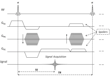
Figure 1.1: A generic SPGR pulse sequence diagram. Here an RF pulse with 𝛼 flip angle is applied. GSS is the slice-encode gradient; GPE is the phase-encode gradient and GFE is the frequency-encode gradient. TE is the echo-time of the acquired signal; TR is the repetition time. Spoilers are indicated at the end of the TR . ... 8

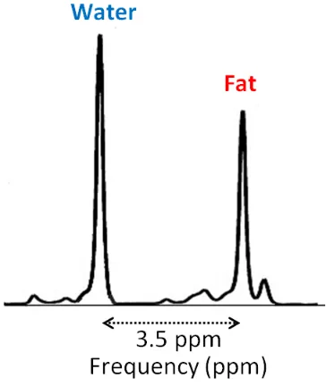
Figure 1.2: A representative frequency spectrum of the MRI signal, showing two main peaks for water and fat, separated by 3.5 ppm ... 10

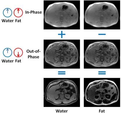
Figure 1.3: The two-point Dixon method reconstructs water and fat images by adding and subtracting in-phase and out-of-phase images, respectively ... 12

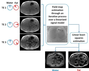
Figure 1.4: Illustration of the IDEAL water/fat separation process ... 15

Figure 1.5: Frequency spectrum of knee subcutaneous fat showing 6 peaks, with the main peak located at ~420 Hz (3.5 ppm) – Figure adapted from [50] ... 18

Figure 1.6: Illustration of the 6-point T2*-IDEAL proposed by

(15)

xiv

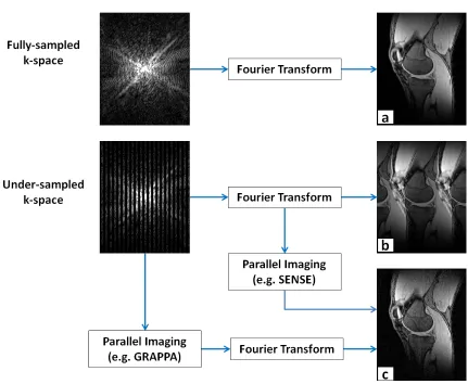
Figure 1.8: (a) A knee image obtained from the Fourier transform of a fully-sampled k-space. (b) Undersampling the k-space results in an aliased image. (c) The image is reconstructed from the undersmapled k-space using Parallel Imaging reconstruction ... 25

Figure 1.9: Left: A discrete flow network problem with a min-cut solution. Right: A Continuous flow network problem. ... 28

Figure 2.1: Water/fat swaps appearing in field map (top), water (left) and fat components (right) ... 44

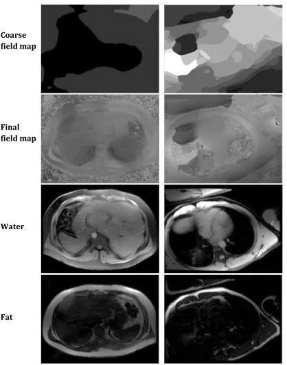
Figure 2.2: Left column: axial abdominal slice, Right column 4-chambers cardiac view. Top to bottom: the coarse estimate of field map from the max-flow stage, final field map after the second stage, water and fat components ... 52

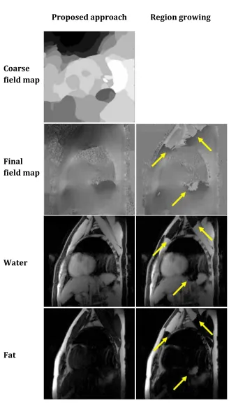
Figure 2.3: Comparison between our approach (left column) and the region-growing method (right column) on a short-axis cardiac image. Yellow arrows indicate the locations of water/fat swaps that have clearly avoided by our method ... 53

Figure 3.1: (a) A point is selected on a 2D axial cardiac image. (b) Neglecting the effect of T2* decay (i.e. R2* = 0), the variation of the signal residuals Γ𝑣(𝜑). (c) By assigning 𝜑𝑣 to its optimal value (-41.5 Hz) and the aliased value (-486 Hz),

the variation of Γ𝑣(𝑅2∗) is drawn with different R2* values ... 67

(16)

xv

water/fat swaps than (a) ... 71

Figure 3.3: Fat water separation in a 4-chamber cardiac slice acquired from a healthy volunteer. (a) Output of the labeling stage showing a coarse estimation of the field map, (b) Final field map after the second stage, (c) Water component, (d) Fat component ... 77

Figure 3.4: Reconstructed data from a 2-chamber cardiac. (a) The labeled field map from the first stage, (b) final field map, (c) fat fraction map and

(d) R2* map ... 78

Figure 3.5: Reconstructed data from an axial abdominal slice. (a) The labeled field map from the first stage, (b) final field map, (c) fat fraction map and (d) R2* map ... 79

Figure 3.6: The reconstruction of the failure case using Max-IDEAL (a), the graph-cut method (b) and the FLAME technique (c). Left to right: field map, water, fat and fat fraction map ... 80

Figure 3.7: Reconstruction of a selected slice from a case provided by the ISMRM 2012 challenge with the labeling approach in [15] (a) and the proposed method (b) ... 81

(17)

xvi

map, water, fat and fat fraction map ... 84

Figure 3.10: Reconstruction of a case from ISMRM 2012 challenge with (a) T2* applied in both stages of the approach, and (b) T2* incorporated only in the second stage (T2*-IDEAL). The reconstruction fails in case T2* decay is not considered in the labeling stage ... 87

Figure 3.11: An example of the boundary artifact appearing in an axial abdominal slice. This artifact is induced around the bowels where very low signal is received ... 89

Figure 3.12: The effect of applying different smoothness levels on the

reconstruction of a case from ISMRM 2012 challenge: (a) β=0.2 was insufficient to remove water/fat swaps; successful reconstruction can be achieved in (b) β = 0.5 and (c) β = 2; (d) Oversmoothed initial field map with β = 4 causes water/fat

artifacts as noted by the arrow. The ASF was not applied in this reconstruction in order to solely examine the effect of the smoothness parameter ... 91

Figure 4.1: (a) A representative diagram of the unipolar sequence. All echoes are acquired with the same readout gradient polarity (positive). Here all echoes are acquired in a single TR (single shot). (b) A representative diagram of the conventional bipolar sequence. Odd echoes are acquired with positive polarities while even echoes have negative polarities. The bipolar acquisition in (b) necessitates employing post-processing phase and magnitude correction algorithms before water/fat separation ... 103

(18)

xvii

centre lines are fully-acquired with both schemes ... 104

Figure 4.3: The reconstruction pipeline for the interleaved bipolar acquisition. The centre of k-space acquired with a positive polarity is used in the self-calibrated parallel imaging reconstruction of the positive lines, and vice-versa for the negative lines ... 105

Figure 4.4: Fat fraction images (ranging from 0% to 5%) of a pure-water phantom from unipolar (a) and interleaved bipolar (b) axial acquisitions. Phase errors from the readout gradient cause fat fraction bias in the unipolar acquisition, while the errors were negligible in the interleaved bipolar results ... 109

Figure 4.5: Results from a coronal acquisition of the phantom set. (a) Fat fraction map of the phantom set with the locations of the 5 vials of different fat fractions indicated. (b) Differences between the true and the measured values from the two sequences, demonstrating accurate fat quantification obtained using the interleaved bipolar compared to the unipolar sequence . ... 109

Figure 4.6: Water and fat images of a volunteer’s knee were obtained with the interleaved bipolar (upper row) and the unipolar sequence (lower row). SNR efficiency maps in (b) and (d) are scaled from [0, 1]. The 2 ROIs in (e) were used for the fat quantification results reported in the text, and demonstrated that accurate fat fractions were obtained with the 2 sequences. However, the SNR efficiency maps (b and d) show that higher SNR efficiency was obtained with the bipolar sequence . ... 110

(19)

xviii

fraction was obtained with the interleaved bipolar sequence ... 111

Figure 4.8: SNR maps of the 2nd echo (a), the water (b) and the fat (c) images from the interleaved bipolar (upper row) and the unipolar (lower row) sequences, respectively. Higher SNR was obtained in all the images with the proposed bipolar sequence ... 112

Figure 5.1: The water component (upper row) and its corresponding SNR efficiency map (lower row) from the four sequences. The interleaved bipolar sequences (B and D) demonstrate higher SNR efficiency compared to the corresponding unipolar sequences (A and C) ... 127

Figure 5.2: The fat component (upper row) and its corresponding SNR efficiency map (lower row) from the four sequences. The interleaved bipolar sequences (B and D) demonstrate higher SNR efficiency compared to the corresponding unipolar sequences (A and C) ... 128

Figure 5.3: The fat fraction images from the four sequences. (A) Unipolar, (B) Interleaved bipolar, (C) Accelerated unipolar, (D) High resolution interleaved bipolar. Accurate fat fraction was obtained with the interleaved bipolar sequences compared to their corresponding unipolar sequences ... 129

(20)

xix

List of Abbreviations

2D

Two dimensional

3D

Three dimensional

BW

Acquisition

bandwidth

EPI

Echo-planar imaging

ETL

Echo-train length

FLAME

Fat-likelihood analysis for multi-echo signals

FOV

Field of view

FT

_{Fourier transform}

GE

Gradient-echo sequence

GRAPPA

Generalized auto-calibrating partially parallel

acquisitions

GPGPU

General-purpose computing on graphics processing

unit

(21)

xx

IDEAL

Iterative decomposition of water and fat with echo

asymmetry and least-squares

MDL

Minimum description length

MRI

Magnetic resonance imaging

NEX

Number of excitations

NSA

Number of signal averages

R

2*

Effective transverse relaxation time

RF

Radio frequency

ROI

Region of interest

SE

Spin-echo sequence

SENSE

Sensitivity encoding (parallel imaging reconstruction)

SNR

_{Signal to noise ratio}

SPGR

Spoiled gradient-recalled echo

ΔTE

Inter-echo spacing

T

Tesla

T

1

Longitudinal relaxation time

TE

Echo-time

(22)

Chapter 1 Introduction

1.1 Motivation

Fat is an important diagnostic marker in many clinical applications, including liver [1], cardiac [2, 3], musculoskeletal system [4, 5], kidney [6], bone marrow [7, 8], measurement of total body fat [9], quantifying visceral adipose tissue [10], as well as distinguishing between white and brown adipose tissue [11, 12]. In liver applications for example, non-alcoholic fatty liver disease (NAFLD), one of the most common chronic liver conditions, is characterized by fatty infiltration of the liver [13, 14], and quantification of fat is necessary in the diagnostic process. Fat signal is also a relevant diagnostic marker of cardiac diseases such as myocardial fatty infiltration [15], which is associated with sudden cardiac death [16], arrhythmogenic right ventricular dysplasia (ARVD) [17] and chronic myocardial infarction [18]. Additionally, interest in measuring the epicardial and intra-thoracic fat has markedly increased in the last decade [2, 19], with some studies suggesting

(23)

such fat deposits to be strongly correlated with the presence of coronary artery disease [20].

Among different medical imaging modalities, Magnetic Resonance Imaging (MRI) is well suited for fat quantification for its ability to separate the signals from water and fat in the human body. Uniquely, MRI can exploit small differences in the frequency of signals received from different chemical species to generate individual images of each species. Water and fat are the main sources of signal in MR images for most clinical applications. MRI can distinguish between water-based and fat-based tissues producing fat-suppressed (water-only) and water-suppressed (fat-only) images, which are commonly needed in clinical diagnosis.

Fat quantification is usually performed in terms of fat fraction, which is the ratio of the fat signal to the total signal from both water and fat. A typical example is the measurement of liver fat in NAFLD patients, where the fat fraction of healthy liver should not exceed 5% [13]. Therefore, accurate and precise fat measurement is required. Several confounding factors can bias the fat fraction measure and must be considered during signal acquisition and reconstruction. These factors include, but not limited to, the tissue-specific relaxation times (such as T1 and T2*) and the inhomogeneities of the main magnetic field.

(24)

1.2 Magnetic Resonance Imaging

1.2.1 Principles of Magnetic Resonance Imaging

MRI relies on a strong magnetic field,𝐵0, which polarizes the nuclear spins in

parallel and anti-parallel directions with respect to the main magnetic field. In the presence of an external magnetic field, the nuclear spins are polarized along the main field, leading toa net magnetization in the parallel direction. The precession frequency of the nuclear spins can be described by the Larmor equation as follows:

𝜔0 = 𝛾𝐵0 (1.1)

where𝜔0 is called the Larmor frequency and 𝛾 is the gyromagnetic ratio of the

nucleus being imaged. Most of the clinical MRI scans targets the Hydrogen proton 1_H as it is the dominant nucleus in the human body. For 1_H,_𝛾_{is equal to 2.68x10}8 rad/s/Tesla. The commonly used value is 𝛾 =𝛾/(2𝜋) = 42.6 MHz/Tesla.

The net magnetization, 𝑀, resulting from the polarized spins cannot be detected as long as it aligns along the direction of the main magnetic field. Hence, an additional magnetic field,𝐵1, is applied to tilt the magnetization away from the 𝐵0direction.

This process can be described through the Bloch equation as follows:

𝑑𝑀��⃗

𝑑𝑡 = 𝑀��⃗ ×𝐵�⃗ (1.2)

where

𝐵�⃗= 𝐵��⃗0+ 𝐵��⃗1 (1.3)

Equation 1.2 is a simplified version of the Bloch equation where the relaxation times are neglected. The 𝐵1 magnetic field is generated by a radiofrequency pulse (RF

pulse) applied through a ‘transmit’ coil tuned at the Larmor frequency. In equilibrium, 𝑀is aligned with 𝐵0along the longitudinal (𝑧̂) direction. As of Equation

1.2, once the RF pulse is applied along 𝑥�or 𝑦�direction, the magnetization vector

(25)

plan (x-y plan). The tipping (or flip) angle is determined by the magnitude of the RF pulse, 𝐵1, and its duration 𝜏, such that:

𝛼 = 𝛾 � 𝐵1(𝑡) 𝜏

0 (1.4)

Following the RF excitation both the longitudinal and transverse components of the magnetization start to relax via two mechanisms: First the longitudinal relaxation described by the time constant 𝑇1, where the magnetization starts to relax back to

its equilibrium state along the 𝑧̂direction. This is called the spin-lattice relaxation as it results from the interaction between the spins and the surrounding lattice. The second relaxation process is a transverse relaxation resulting from the interactions between spins, hence called the spin-spin relaxation. It results from the ‘dephasing’ of the spins and is governed by a time constant 𝑇2. The two relaxation processes can

be described through the Bloch equation:

𝑑𝑀��⃗

𝑑𝑡 = 𝑀��⃗ ×𝐵�⃗ −

𝑀𝑥𝑥�+ 𝑀𝑦𝑦�

𝑇2 −

(𝑀𝑧− 𝑀0) 𝑧̂

𝑇1 (1.5)

Shortly after the RF excitation, the signal is sampled at a time ‘TE’ (or echo time) and detected through a ‘receiver’ coil. The detected signal is proportional to the magnitude of the transverse component of the magnetization,𝑀𝑥𝑦, and can be

derived from the Bloch equation above (Equation 1.5). For example, if a pulse with

𝜋/2 flip angle is applied, the initial magnetization 𝑀𝑖𝑛𝑖𝑡will be fully tipped to the

transverse plan. Ideally, immediately after the RF pulse at time 𝑡 = 0, the magnetization vector 𝑀𝑧(0) = 0 and 𝑀𝑥𝑦= 𝑀𝑖𝑛𝑖𝑡. The magnetization vectors at

time 𝑡 can be then derived from Equation 1.5, resulting in the following components:

𝑀𝑧(𝑡) = 𝑀𝑖𝑛𝑖𝑡�1− 𝑒−𝑡 𝑇�1� (1.6)

(26)

Hence the magnitude of the detected signal at time ‘TE’ will be proportional to

𝑀𝑖𝑛𝑖𝑡.𝑒−𝑇𝐸 𝑇�2. If we started from the equilibrium state, then 𝑀𝑖𝑛𝑖𝑡 = 𝑀0. The

received signal is therefore proportional to the bulk spin density, 𝜌, in the excited volume.

1.2.2 Spatial Encoding

So far we have introduced two sources of magnetic fields, the main magnetic field,𝐵0, and the RF pulse. In order to ‘encode’ the spatial position of received signal,

additional magnetic fields, called gradients, are employed. A gradient is a linearly varying magnetic field added to the static field to distinguish the spins along a certain direction. For example in the 𝑥-direction it is given by:

𝐵(𝑥,𝑡) = 𝐵0+𝑥𝐺𝑥(𝑡) (1.8)

where 𝐺𝑥is a constant gradient in the 𝑥-direction. The precession frequency will

therefore vary along the𝑥-diretion. Demodulating the Larmor precession, the phase accrual occurring due to the applied gradient is given by:

𝜑𝑥(𝑥,𝑡) =−𝛾𝑥 � 𝐺𝑥(𝑡′) 𝑑𝑡′ 𝑡

0 (1.9)

Similarly, a gradient is added in the 𝑦-direction, also causing an accumulation of phase along this direction. For a 2D acquisition, the received signal is now the product of the excited spin density with the gradients-induced phase terms along the two directions:

𝑆(𝑥,𝑦) ∝ ∬ 𝜌(𝑥,𝑦)𝑒−𝑖�𝜑𝑥(𝑥,𝑡) +𝜑𝑦(𝑦,𝑡)�_𝑑𝑥_𝑑𝑦_(1.10)

Defining 𝑘𝑥and 𝑘𝑦as the spatial frequencies in the𝑥- and 𝑦- directions respectively,

Equation 1.10 can be written as follows:

(27)

where

𝑘𝑥 =₂𝛾_{𝜋 � 𝐺}𝑥(𝑡′) 𝑑𝑡′ 𝑡

0 (1.12)

𝑘𝑦 = ₂𝛾_{𝜋 � 𝐺}𝑦(𝑡′) 𝑑𝑡′ 𝑡

0 (1.13)

Neglecting the relaxation terms, Equation 1.11 is the form of a 2D Fourier transform (FT) of the spin density𝜌(𝑥,𝑦). Hence, an inverse 2D FT of the encoded signal will be a representation of the distribution of the underlying spin density, i.e.

𝜌(𝑥,𝑦) =𝐹𝑇−1_{�𝑆�𝑘}

𝑥,𝑘𝑦��.

Equation 1.11 shows that MRI spatial encoding is achieved in terms of 𝑘𝑥and 𝑘𝑦, i.e.

the signal data is a representation of the spatial frequencies of the spin density, and is therefore called 𝑘-space. The 𝑘𝑥direction is called the frequency encode or the

readout direction, while the𝑘𝑦is called the phase encode direction. For a 3D

acquisition, another phase encode direction, 𝑘𝑧, is employed through the linear

gradient𝐺𝑧. Most of the clinical scans follow a Cartesian trajectory during the

acquisitions, where one phase-encode line is acquired at each repetition time (TR). Before acquiring the signal at each line, the y- gradient is modified one step (Δ𝑘𝑦) to

target a new spatial location in the phase-encode direction. The 𝑥-gradient, however, is turned on during the signal acquisition to capture the samples in the readout direction. The length of the readout for one echo depends on the receiving bandwidth and the number of samples in the frequency-encode direction, where the receiving bandwidth defines the number of samples collected per unit time.

(28)

1.2.3 Gradient-echo Sequences

Although water/fat imaging can be performed with SE-based sequences, GE-based sequences are usually used as they are generally faster, particularly for 3D imaging [21]. In contrast to SE, GE sequences do not employ RF refocusing pulses (𝜋-pulse) and hence shorter TRs can be achieved as there is no need to wait for the

𝑇1 recovery time. The TR is directly proportional to the scan time, so shorter

acquisitions are achieved with GE. This is particularly important when time-restricted water/fat acquisitions are required, for example whole-liver fat quantification in a single breath-hold (~20s).

As refocusing pulses are not applied, B0 field inhomogeneities cause an additional source of dephasing, in addition to the spin-spin relaxation. In other words, the time constant 𝑇2in the signal equation will be replaced by 𝑇2∗, such that:

1⁄𝑇2∗ = 1⁄𝑇2′+ 1⁄𝑇2 (1.14)

where 𝑇2′is the relaxation factor resulting from the local field inhomogeneities. In

contrast to 𝑇2relaxation which is an intrinsic property of the tissue, 𝑇2′depends on

different factors including: the shimming of the magnet as well as variations in the magnetic susceptibility of the tissues within the patient [22, 23]. Measuring 𝑇2∗is

useful in various clinical applications, for example, detecting hemorrhage [24] and assessing the iron overload in liver diseases [25]. However, as 𝑇2∗relaxation is

shorter than𝑇2, the transverse magnetization decays faster. This makes GE images

more prone to signal loss artifacts than spin-echo sequences [21, 23].

(29)

𝑆= 𝑀0

�1− 𝑒−𝑇𝑅�𝑇1�

�1−cos𝛼 . 𝑒−𝑇𝑅�𝑇1�.𝑒 −𝑇𝐸_𝑇

2∗ �

. sin𝛼 (1.15)

In order to achieve zero transverse magnetization before each RF pulse, ‘spoiling’ the signal from previous excitations is necessary. The sequence is therefore called spoiled gradient-echo or SPGR. RF spoiling is a commonly used spoiling technique; it employs different phases for the RF pulse at each TR. Another spoiling approach is to apply additional gradient lobes on the 3 axes at the end of the TR to ensure the spoiling in all the directions. This requires that the area of any of the 3 gradients must not vary from TR to TR; otherwise the spoiling will be spatially dependent. The pulse sequence diagram of SPGR is shown in Figure 1.1

Figure 1.1: A generic SPGR pulse sequence diagram. Here an RF pulse with 𝛼flip angle is applied. GSS is the slice-encode gradient; GPE is the phase-encode gradient and GFE is the frequency-encode gradient. TE is the echo-time of the acquired signal;

(30)

1.3 Water/Fat Imaging

Water and fat protons are the main sources in 1_{H proton MR images. The} suppression of fat signal is desirable whenever it obscures the underlying pathology as in breast imaging [26], head and neck imaging [27] or cardiac imaging [28]. On the other hand, detection of the fat signal is of a clinical interest in other applications such as the quantification of liver fat deposition in non-alcoholic fatty liver diseases (NAFLD) [14, 25, 29], diagnosis of myocardial fatty infiltration [15] and detection of renal angiomyolipoma [6]. In such applications, suppressing the water signal is instead required. Uniquely, chemical-shift-encoded water/fat imaging allows the separation of water and fat, while preserving both signals. It provides a water-only (fat-suppressed) and fat-only (water-suppressed) images, which makes it useful for a wide variety of clinical needs.

1.3.1 Chemical-Shift-Encoded Water/Fat Imaging

This technique exploits the frequency spectrum of fat and water signals. Because of the difference of electronic shields, the protons of fat molecules ‘see’ different magnetic field than what is observed by the protons in water molecules. This gives rise to a difference in the spectral components of the MR signal, with the main peak of the fat signal separated by approximately 3.5 parts-per-million (ppm) – Figure 1.2. This difference is termed the chemical-shift and is equal to ~210 Hz at 1.5 Tesla or ~420 Hz at 3 Tesla.

(31)

the problem for the two unknown species and obtain an independent image for each species.

Figure 1.2: A representative frequency spectrum of the MRI signal, showing two main peaks for water and fat, separated by 3.5 ppm

Chemical-shift imaging can be combined with any pulse sequence including steady-state free-precession (SSFP) [31], fast spin-echo (FSE) [27, 32]and spoiled gradient-echo (SPGR) [33]. Also, its ability to generate fat-only and water-only (fat suppressed) images is a key advantage that made it widely used for water/fat imaging. In general, this approach can be described by a simplified model as follows:

𝑆𝑣(𝑡𝑛) =𝜌𝑤,𝑣+ 𝜌𝑓,𝑣𝑒𝑖2𝜋𝛿𝑡𝑛 (1.16)

where 𝑆𝑣(𝑡𝑛) is the signal acquired at voxel 𝑣at time 𝑡𝑛where 𝑛= 1, . .𝑁;

𝜌𝑤,𝑣represents the water component and 𝜌𝑓,𝑣is the fat component; 𝛿is the

chemical-shift difference (~420 Hz at 3T). This model has neglected other factors as

(32)

In the last decade, extensive research has been conducted on Dixon-based methods showing its robustness in separating water and fat, offering unique advantages over other approaches. The next sections we will describe different Dixon-based methods in further detail.

1.3.2 Two-Point Dixon

Dixon first proposed his method by acquiring 2 images at 2 different TEs [34]. The first TE is adjusted to acquire an “in-phase” image where water and fat have the phase value. The second acquisition is an “out-of-phase” one where water and fat exhibit a 𝜋phase difference. Water and fat components can be therefore obtained by simply adding and subtracting the two acquired images - Figure 1.3, leading to:

𝜌�𝑤 =1₂�𝑆�𝑡𝑖𝑝�+𝑆�𝑡𝑜𝑝�� (1.17)

𝜌�𝑓 =1₂�𝑆�𝑡𝑖𝑝� − 𝑆�𝑡𝑜𝑝�� (1.18)

where 𝑡𝑖𝑝and 𝑡𝑜𝑝are the TE values where fat and water are in-phase and

(33)

(34)

1.3.3 Three-point Dixon

Glover and Schneider proposed the three-point Dixon method to estimate the magnetic field inhomogeneities [36]. Using a spin-echo sequence, they acquire three images at 3 different TEs where fat and water exhibit relative phase-shifts of −𝜋, 0 and𝜋. The signal model from the 3 acquisitions can be described as follows:

𝑆(𝑡−𝜋) =�𝜌𝑤 − 𝜌𝑓�𝑒𝑖(𝜃0−𝜃) (1.19)

𝑆(𝑡0) =�𝜌𝑤+ 𝜌𝑓�𝑒𝑖𝜃0 (1.20)

𝑆(𝑡𝜋) =�𝜌𝑤 − 𝜌𝑓�𝑒𝑖(𝜃0+𝜃) (1.21)

where 𝜃0 is an unknown systematic phase offset, while 𝜃 is the unknown phase term

resulting from the field inhomogeneities. After demodulating 𝜃0of all the 3

acquisitions using Equation 1.20, water and fat components can be derived as follows:

𝜌𝑤 =�𝑆 ′₍_𝑡

0) + 𝛽�𝑆′(𝑡𝜋) . 𝑆′(𝑡−𝜋)�

2 (1.22)

𝜌𝑓 =�𝑆 ′₍_𝑡

0)− 𝛽�𝑆′(𝑡𝜋) . 𝑆′(𝑡−𝜋)�

2 (1.23)

where 𝑆′_{is the signal after omitting}_𝜃

0and 𝛽 = ±1 is a switch function for sign of

the complex square root. However, in order to assign the correct 𝛽sign, a phase unwrapping algorithm is required. The main limitation of Glover and Schneider’s technique is that it restricts the acquisition to −𝜋, 0 and𝜋. A more flexible version of the three-point Dixon was proposed by Xiang and An [37] where the 3 acquisitions are acquired at uniformly-spaced TE shifts. The field inhomogeneity𝜑 is then estimated through a quadratic equation in the phasor term𝑒−𝑖2𝜋𝜑∆𝑡_{. Similar to}

(35)

1.3.4 IDEAL

A novel perspective to the three-point Dixon was introduced by Reeder et al. [38] based on a maximum likelihood estimation of the signal. They introduced the “Iterative Decomposition of water and fat with Echo Asymmetry and Least-squares estimation” (IDEAL) where a nonlinear least-squares fitting is performed at each voxel. A general description of the acquired signal at voxel,𝑣, can be given by re-writing Equation 1.16 as follows:

𝑆𝑣(𝑡𝑛) =�� 𝜌𝑐,𝑣𝑒𝑖2𝜋𝛿𝑐𝑡𝑛 𝐶

𝑐=1

� .𝑒𝑖2𝜋𝜑𝑡𝑛 (1.24)

Where 𝐶 is the number of species, 𝜌𝑐,𝑣is a complex-valued chemical species with

𝛿𝑐 representing its chemical-shift from the main water-peak (in Hz) and 𝜑is a map

of the field inhomogeneities, so called field map. The key point of IDEAL is solving the problem in an iterative linearization procedure of the signal equation – Figure 1.4. The approach can be summarized:

a. An initial estimate is given to𝜑. Usually it is set to zero.

b. The chemical species can be then estimated directly through solving a linear least-squares problem.

c. The estimates �𝜑� 𝜌�, 𝑐,𝑣�,𝑐 = 1, . . ,𝐶 are then fed into a linearized signal

model, where 𝑒𝑖2𝜋∆𝜑𝑡𝑛 is approximated through Taylor expansion

by 1 +𝑖2𝜋∆𝜑𝑡𝑛 .

d. The signal residues from these estimates are then calculated

e. A new value for the field map is calculated 𝜑𝑖+1= 𝜑𝑖 +∆𝜑, where 𝑖is

the iteration number.

f. Step (b-e) are repeated until ∇𝜑converges (e.g. < 1 Hz).

g. Calculate the final estimates of 𝜑and 𝜌𝑐,𝑣for all chemical species.

(36)

IDEAL has several advantages over previous approaches: 1) it can be used with arbitrary TEs; 2) it can be combined with any imaging sequence; 3) it works for any number of chemical species i.e. not restricted to water/fat applications; 4) complex-valued chemical species are estimated, which enhances the effective number of signal averages (NSA) of the reconstruction (refer to 1.3.5 for more details). On the other hand, a major drawback of IDEAL is the initial value required for the field map𝜑; If not correctly estimated for each voxel, the algorithm will converge into local minima and wrong estimates of water/fat will be obtained. Hence, IDEAL will fail in cases where large inhomogeneities are encountered as it does not enforce any global solution to the iterative procedure. Several techniques have been proposed to resolve the large variations in the field map [9, 39-46]. Although some methods have demonstrated the ability to address challenging cases, an ultimate solution to the field map estimation problem has yet to be explored. In Chapters 2 and 3 we will propose new methods to overcome the drawbacks of IDEAL.

(37)

1.3.5 Characterization of Noise Performance

The noise performance of water/fat separation methods rely on multiple of acquisition and reconstruction parameters [47]. The common metric to evaluate the noise performance is the effective number of signal averages (NSA) given by

𝑁𝑆𝐴= 𝜎_𝜎2

𝑝2 (1.25)

Here 𝜎2_and _𝜎

𝑝2are the variance of the noise in the source image and the

reconstructed fat (or water) image, respectively. The minimum achievable 𝜎𝑝2 is

calculated using the Cramér-Rao bound, which is defined as the lower bound on the variance of an unbiased estimate. Hence it can be used to optimize the acquisition parameters to attain the highest noise performance. Pineda et al. [47] showed that for 3-point Dixon, echo-shifts of (𝜋₆ +𝜋𝐾,𝜋₂+𝜋𝐾,7𝜋₆ +𝜋𝐾) achieves best theoretical performance using the signal model of Equation 1.24 for water and fat species. In theory, the maximum achievable NSA for n-point acquisition is n. NSA depends mainly on a number of factors: the number of echoes, the first echo, the echo-shifts and the number of unknown parameters to be estimated in the reconstruction [47,

(38)

1.4 Quantitative Fat Imaging

Fat quantification is usually performed in terms of fat fraction, which is the ratio of the fat signal to the total signal from both water and fat. Several confounding factors can bias the fat measurement and must be considered in the reconstruction. Once these factors are addressed, the fat fraction will be equivalent to what is referred to as proton density fat-fraction (PDFF) which is defined as the ratio of density of mobile protons from fat to the total density of mobile protons from fat and water. PDFF is currently considered the most practical and meaningful MR-based biomarkers for fat quantification [49]. Current research is seeking its standardization for clinical diagnosis.

1.4.1 Multi-peak Fat Spectrum

The signal model presented in Equation 1.16 and Equation 1.24 assumes that fat exhibits one peak in the frequency spectrum of the MR signal. However due to the complex nature of fat molecule, its protons vary in their precession frequencies. It was shown that the fat spectrum can have up to 6 peaks with different amplitudes – Figure 1.5. A significant bias in the fat fraction measurements will occur if only the main peak is considered [50]. Therefore, a multi-peak fat spectrum is included in the signal equation as follows:

𝑆𝑣(𝑡𝑛) =�𝜌𝑊,𝑣+𝜌𝐹,𝑣 .� 𝛼𝑚.𝑒𝑖2𝜋𝛿𝑚𝑡𝑛 𝑀

𝑚=1

�.𝑒𝑖2𝜋𝜑𝑣𝑡𝑛 (1.26)

where 𝑀is the number of fat peaks; 𝛿𝑚 is the frequency of the 𝑚-th peak with its

(39)

Figure 1.5: Frequency spectrum of knee subcutaneous fat showing 6 peaks, with the main peak located at ~420 Hz (3.5 ppm) – Figure adapted from [50].

Equation 1.26 now includes additional 2M unknowns: frequencies and amplitudes of the fat peaks. Fortunately, the frequencies are well documented in the literature [51-53] and can be assumed to be constant. There are two approaches to obtain the amplitudes: self-calibrated and pre-calibrated methods. In the self-calibrated method different fat peaks are treated as different chemical species and hence large number of echoes (images) are required to solve Equation 1.26. For instance Yu et al. [50] used 16 echoes in order to obtain an accurate fit for all the peaks. On the other hand, the pre-calibrated approach assumes predetermined amplitude values for the fat peaks and hence it leads to the same number of unknowns. Several studies have shown that including the multi-peak fat spectrum improves the accuracy of estimating the fat fraction compared to the single peak approach [14, 25,

(40)

1.4.2 Effect of T

2*

Relaxation

In Equation 1.24 and Equation 1.26, T2* decay was assumed to be negligible. However, this assumption can lead to substantial errors in the fat fraction estimate [14, 54, 55], particularly with rapid T2*. Additionally, T2* itself might be of diagnostic interest in some cases, such as hepatic iron overload, as R2* (1/T2*) is strongly correlated to the iron deposition. Likewise, the presence of fat can lead to wrong T2* estimates. Therefore, methods that consider single-T2* [54] and dual-T2* [56] decays during water/fat reconstruction have been introduced. The latter approach estimates two T2* values for water and fat respectively, while the single-T2* approach ignores that difference and a single combined decay is deduced at each voxel. In theory, fat fraction bias should decrease with dual-T2*[55]; however, the noise performance significantly degrades as more unknown parameters are included in the reconstruction process [48]. Consequently dual-T2* models result in noisy estimates of fat fraction. In practice, studies have shown that single-T2* modeling is more accurate than dual-T2* model for fat quantification, even with high fat concentration [57].

(41)

(42)

1.4.3 T

1

-related bias

Fat has shorter T1 relaxation time than water. This may result in a dissimilar weighting between water and fat signals in the acquired image, as the signal received from fat protons is higher compared to that received from water. Consequently, significant bias in the fat fraction measurements can occur [58]. Accurate PDFF quantification necessitates the correction of T1-related bias [49, 58,

59].

(43)

1.4.4 Eddy Currents

To shorten the acquisition time, multi-point chemical-shift-encoded sequences perform multiple readout gradients in each TR – Figure 1.7. Eddy currents are generated at each time the gradients are switched ‘on’ and ‘off’ producing phase errors in the acquired signals. In a multi-echo SPGR acquisition, the gradient waveform preceding the first readout is different from the waveforms preceding the other echoes. Hence, the generated eddy currents and subsequently the resulting phase errors are different in the first echo from the rest of the echoes. These asymmetric phase errors affect the water/fat separation process, leading to fat-fraction bias. To address this problem, magnitude-based reconstruction is used, where the phase information is omitted. This leads to significant noise amplification in the fat fraction image compared to the complex-based reconstruction where the complex signals are considered [48].

Figure 1.7: Three readout gradients are applied in one TR to acquire 3 echoes.

(44)

This method has led to further SNR improvement over the hybrid method. Recently Wade et al. [64] suggested modifying the waveforms of the readout gradient to generate similar eddy currents at the first echo as the rest of the echoes. This will compensate for the fat fraction bias as the phase errors will be approximately the same at all the echoes. However, SNR loss might occur from the insertion of an additional waveform before the first echo. We address the eddy currents-induced fat fraction bias with our new acquisition strategy proposed in Chapter 4.

1.4.5 Noise-related bias

Fat fraction bias might also occur when one of the species is at very low concentrations, due to noise amplification. Liu et al. [60] addressed this problem by using the ‘phase-constrained’ hypothesis where fat and water are assumed to have same phase at TE=0. Hence, instead of using the magnitude of fat and water signals to calculate the fat fraction, complex values will be used, such that 𝐹𝐹 =

𝑆𝑓⁄�𝑆𝑓+𝑆𝑤�for fat-dominant-pixels and 𝐹𝐹 = 1− �𝑆𝑤⁄�𝑆𝑓+𝑆𝑤�� for

water-dominant pixels, where 𝑆𝑓and 𝑆𝑤are the complex signals of fat and water,

respectively. This approach has shown to overcome the bias occurring at very low and very high fat concentrations.

1.4.6 Temperature-related bias

(45)

1.5 Parallel Imaging

In general, water/fat imaging requires lengthy acquisitions. Hence, for time-restricted applications, accelerated data acquisition is required. The most common acceleration technique in clinical practice is parallel imaging [66-70].

For a 2D acquisition the scan time is calculated as 𝑡= 𝑁𝑆𝐴 .𝑁𝑦 .𝑇𝑅, where NSA is

the number of signal averages and 𝑁𝑦 is the number of phase encodes. Hence for a

prescribed TR, the fewer phase encodes the shorter the acquisition time will be. However, this will violate Nyquist criterion in k-space, causing aliasing artefacts in the image domain - Figure 1.8(b). Parallel imaging techniques address this problem by recovering the missing data from subsampled k-space and hence allow aliasing-free accelerated acquisitions. Reconstruction techniques can either recover the omitted data in k-space (e.g. GRAPPA) [66, 67, 69], or un-fold the aliased images in image-domain (e.g. SENSE) [70, 71] – Figure 1.8. For 3D imaging, acceleration can be achieved in both the phase and the slice directions by acquiring fewer slice/phase encodes and recovering them in the reconstruction. This will allow even shorter acquisition times.

The key for parallel imaging is taking advantage of a phased-array of coils. In fact, each coil has a non-uniform receive profile - known as coil sensitivity - which is used as calibration data in the reconstruction. Parallel imaging reconstruction techniques, therefore, employ the calibration data to recover the missing slice/phase encodes, whether in k-space or image-domain.

(46)

In chapter 4 of this dissertation we will use conjugate-gradient SENSE for parallel imaging reconstruction [71]. This is an image-based reconstruction technique that uses an iterative approach to un-alias the acquired undersampled data.

Figure 1.8: (a) A knee image obtained from the Fourier transform of a fully-sampled k-space. (b) Undersampling the k-space results in an aliased image. (c) The image is

(47)

1.6 Network Optimization Problems

Resolving the correct field map inhomogeneities in Equation 1.26 is a challenging problem that becomes even more complicated when the confounding factors mentioned above are included in the signal equation. To address this problem, sophisticated optimization techniques can be employed. One of the main branches of mathematical optimization is network optimization techniques, which are employed in Chapters 2 and 3 to estimate the magnetic field inhomogeneities.

1.6.1 Terminology

Basically, a network is defined as a graph constituted of two main objects: nodes and edges. For instance if an image is mapped through a network, each pixel is represented by a node, while weighted edges connect each pixel to other pixels in a local neighbourhood. Moreover, two special nodes are added, a sink node and a source node. The source and sink nodes are connected to all the other nodes in the graph – Figure 1.9.

A flow in a network is simply a quantity that is flowing in an edge from one node to another. Mathematically, a flow of an edge is just a scalar number added on it. A flow can have negative values, where in this case it flows in the opposite direction to the edge. There are two main constraints on the flows of the network: capacity constraints and flow conservation. To define them let’s assume we have a graph (𝑉,𝐸), where 𝑉and 𝐸are the nodes and the edges, respectively. The grid also has two terminal nodes, a sink 𝑡and a source𝑠. There are three sets of flows: source flows, 𝜌𝑠, from the source node 𝑠to each node in the grid; sink flows, 𝜌𝑡, from each

node into the sink node𝑡; and spatial flows 𝑞 between the nodes of the grid. The capacities constraining the flows in the network are defined as follows:

(48)

where𝐶𝑠(𝑣), 𝐶𝑡(𝑣) and 𝐶(𝑣) are the capacities of the corresponding flows. When a

spatial flow 𝑞(𝑒) over the edge 𝑒 ∈ 𝐸reaches its maximum capacity, it is called a ‘saturated’ flow.

The other constraint is the flow conservation, which is defined at node 𝑣 ∈ 𝑉\{𝑠,𝑡}

as follows:

� � 𝑞𝑒(𝑣) 𝑒∈𝐼(𝑣)

� − 𝜌𝑠(𝑣) + 𝜌𝑡(𝑣) = 0 (1.27)

where 𝐼(𝑣) ⊂ 𝐸is the set of the neighbour edges of the node 𝑣. In other words, this constraint states that the total flow departing from the node must be balanced by the arriving flow at the node. By definition, only the source and sink nodes are exempted from this constraint. The flow conservation and the capacity constraints are important conditions that will control the solution of max-flow problems, described next.

1.6.2 Min-cut / Max-flow problem

In a graph network, each edge has a cost. A cut that separates the source node from the sink node will have a total cost equal to the sum of all the edges it passed through. The minimum-cut (min-cut) problem consists of finding the cut that has the lowest cost – Figure 1.9. Finding the optimal solution of an optimization problem corresponds to finding the min-cut of its graph-network. The graph-cut algorithm by Boykov et al. [72, 73] is a widely used algorithm to explore the min-cut of a network. Equivalent to the min-cut solution is finding the maximum-flow of the network. In fact, min-cut/max-flow theorem is very popular in network optimization. In max-flow we try to maximize the max-flow from the source node, while maintaining the capacity and the flow conservation constraints, i.e.

max_𝜌

𝑠 � 𝜌𝑠(𝑣) 𝑣∈𝑉\{𝑠,𝑡}

(49)

subject to the constrains mentioned above. The path that allows the maximum flow divergence out of the source node is equal to the minimum cut that separates the source from the sink. There are a growing number of medical applications that rely on min-cut/max-flow approaches as efficient optimization methods.

Figure 1.9: Left: A discrete flow network problem with a min-cut solution. Right: A Continuous flow network problem.

1.6.3 Continuous Max-flow

The max-flow problem formulated in the previous section was introduced in the discrete setting, and can be formulated in the same manner on a continuous domain. Let be a spatial position on a continuous 2D or 3D domain . The flow constraints can be reformulated as follows:

| |

(50)

Where is the divergence of the flow at representing the total spatial flow, which is analogous to the sum operator in Equation 1.28. The continuous max-flow model can now be formulated as follows:

∫

subject to the constraints in Equations 1.29-1.32. By introducing a multiplier to the flow conservation in Equation 1.33, the max-flow model can be re-written as follows:

∫ ∫

| |

(51)

1.7 Thesis Outline

The thesis presents novel acquisition and reconstruction methods for water/fat separation with in-vivo applications on various human organs. Chapter 2, 3 and 4 are based on published peer-reviewed articles to Magnetic Resonance in Medicine (MRM) and Medical Image Computing and Computer Assisted Intervention (MICCAI).

In Chapter 2 a novel water/fat separation technique is introduced. The chapter is adapted from a peer-reviewed paper published in MICCAI 2012 proceedings. The technique estimates magnetic field inhomogeneities that hinder the reconstruction process. In contrast to most of the previous work that rely on spatial smoothness, the presented method uses a labeling model to resolve the ambiguity of the estimation. An initial guess of the field map is generated first then the estimate is subsequently refined using an IDEAL iterative process. The number of labels used to describe the initial estimate is penalized in the cost function to enforce fewer labels. This was shown to reduce the vulnerability of converging to local minima. In-vivo experiments were performed on cardiac and abdominal datasets showing excellent water/fat separation. The results were compared against the commonly-used region-growing method and have demonstrated significant outperformance in case of abrupt changes of magnetic field.

In Chapter 3 an optimized version of the method proposed in the previous chapter is presented. The effect of T2* decay was integrated in the labeling process. The initial

estimate becomes better representative of the signal model and therefore more robust to local minima. In addition, an adaptive spatial filtering was introduced after the labeling procedure to enhance the performance of the method. A continuous max-flow approach was employed to address the labeling model, while T2*-IDEAL is

applied in the second stage; the technique is therefore called Max-IDEAL. In-vivo

(52)

on in-vivo cases with severe inhomogeneities and has demonstrated successful water/fat separation while the other methods failed.

In Chapter 4 a new multi-gradient-echo bipolar acquisition sequence for fat quantification is proposed. This new acquisition strategy is more efficient than the current unipolar sequence currently employed in clinical practice. The sequence applied bipolar gradients at the frequency-encode gradient while alternating the polarity in the temporal dimension as well as the phase-encode dimension. The acquisition and reconstruction pipeline overcomes the bipolar artefacts known to corrupt the water/fat separation procedure. Phantoms and in-vivo experiments demonstrated accurate fat fraction and increased SNR efficiency compared to the established unipolar acquisition. Phase and magnitude artefacts from the bipolar acquisition were eliminated in all experiments.

In Chapter 5 the efficiency of the interleaved bipolar acquisition proposed in the previous chapter is demonstrated in animal experiments. One of the common applications of water/fat separation is to study obesity on animal models. Fat and water images with high spatial resolution are required. Using the interleaved bipolar sequence, the spatial resolution was doubled while keeping the same acquisition time as the standard unipolar sequence. The results also demonstrated higher SNR efficiency of the interleaved bipolar compared to the unipolar sequences.

(53)

References

[1] Alfire, M. E. and Treem, W. R., "Nonalcoholic fatty liver disease," Pediatr Ann,

vol. 35, pp. 290-4, 297-9, Apr 2006.

[2] Iozzo, P., "Myocardial, Perivascular, and Epicardial Fat," Diabetes Care, vol. 34, pp. S371-S379, 2011.

[3] Börnert, P., Koken, P., Nehrke, K., Eggers, H., and Ostendorf, P., "Water/fat‐ resolved whole‐heart Dixon coronary MRA: An initial comparison," Magnetic Resonance in Medicine, vol. 71, pp. 156-163, 2014.

[4] Shin, P. J., Larson, P. E. Z., Ohliger, M. A., Elad, M., Pauly, J. M., Vigneron, D. B., et al., "Calibrationless parallel imaging reconstruction based on structured low-rank matrix completion," Magnetic Resonance in Medicine, vol. 72, pp. 959-970, 2014.

[5] Siepmann, D. B., McGovern, J., Brittain, J. H., and Reeder, S. B., "High-resolution 3D cartilage imaging with IDEAL–SPGR at 3 T," American Journal of Roentgenology, vol. 189, pp. 1510-1515, 2007.

[6] Israel, G. M., Hindman, N., Hecht, E., and Krinsky, G., "The use of opposed-phase chemical shift MRI in the diagnosis of renal angiomyolipomas," American Journal of Roentgenology, vol. 184, pp. 1868-1872, 2005.

[7] Schick, F., Weiss, B., and Einsele, H., "Magnetic resonance imaging reveals a markedly inhomogeneous distribution of marrow cellularity in a patient with myelodysplasia," Annals of hematology, vol. 71, pp. 143-146, 1995.

[8] Schick, F., Einsele, H., Lutz, O., and Claussen, C., "Lipid selective MR imaging and localized 1H spectroscopy of bone marrow during therapy of leukemia,"

(54)

[9] Berglund, J., Johansson, L., Ahlström, H., and Kullberg, J., "Three-point dixon method enables whole-body water and fat imaging of obese subjects,"

Magnetic Resonance in Medicine, vol. 63, pp. 1659-1668, 2010.

[10] Addeman, B. T., Kutty, S., Perkins, T. G., Soliman, A. S., Wiens, C. N., McCurdy, C. M., et al., "Validation of volumetric and single‐slice MRI adipose analysis using a novel fully automated segmentation method," Journal of Magnetic Resonance Imaging, 2014. DOI:10.1002/jmri.24526.

[11] Hu, H. H., Smith, D. L., Nayak, K. S., Goran, M. I., and Nagy, T. R., "Identification of brown adipose tissue in mice with fat–water IDEAL‐MRI," Journal of Magnetic Resonance Imaging, vol. 31, pp. 1195-1202, 2010.

[12] Hu, H. H., Yin, L., Aggabao, P. C., Perkins, T. G., Chia, J. M., and Gilsanz, V., "Comparison of brown and white adipose tissues in infants and children with chemical-shift-encoded water-fat MRI," Journal of Magnetic Resonance Imaging, 2013.

[13] Lall, C. G., Aisen, A. M., Bansal, N., and Sandrasegaran, K., "Nonalcoholic fatty liver disease," Am J Roentgenol, vol. 190, pp. 993-1002, 2008.

[14] Hines, C. D. G., Frydrychowicz, A., Hamilton, G., Tudorascu, D. L., Vigen, K. K., Yu, H., et al., "T1 independent, T2* corrected chemical shift based fat--water separation with multi-peak fat spectral modeling is an accurate and precise measure of hepatic steatosis," Journal of Magnetic Resonance Imaging, vol. 33, pp. 873-881, 2011.

[15] Kellman, P., Hernando, D., and Arai, A. E., "Myocardial Fat Imaging," Current Cardiovascular Imaging Reports, vol. 3, pp. 83-91, 2010.

(55)

[17] Burke, A. P., Farb, A., Tashko, G., and Virmani, R., "Arrhythmogenic Right Ventricular Cardiomyopathy and Fatty Replacement of the Right Ventricular Myocardium Are They Different Diseases?," Circulation, vol. 97, pp. 1571-1580, 1998.

[18] Goldfarb, J. W., Roth, M., and Han, J., "Myocardial Fat Deposition after Left Ventricular Myocardial Infarction: Assessment by Using MR Water-Fat Separation Imaging 1," Radiology, vol. 253, pp. 65-73, 2009.

[19] Verhagen, S. N. and Visseren, F. L. J., "Perivascular adipose tissue as a cause of atherosclerosis," Atherosclerosis, vol. 214, pp. 3-10, 2011.

[20] Bachar, G. N., Dicker, D., Kornowski, R., and Atar, E., "Epicardial Adipose Tissue as a Predictor of Coronary Artery Disease in Asymptomatic Subjects," Am J Cardiol, vol. 110, pp. 534-538, 2012.

[21] Bernstein, M. A., King, K. F., and Zhou, X. J., Handbook of MRI pulse sequences: Elsevier Academic Press, 2004.

[22] Haacke, E. M., Brown, R. W., Thompson, M. R., and Venkatesan, R., Magnetic resonance imaging: Physical principles and sequence design: John Wiley and Sons, 1999.

[23] McRobbie, D. W., Moore, E. A., Graves, M. J., and Prince, M. R., MRI from Picture to Proton: Cambridge University Press, 2006.

[24] Bradley, W. G., "MR appearance of hemorrhage in the brain," Radiology, vol. 189, pp. 15-26, 1993.

(56)

[26] Le-Petross, H., Kundra, V., Szklaruk, J., Wei, W., Hortobagyi, G. N., and Ma, J., "Fast three-dimensional dual echo dixon technique improves fat suppression in breast MRI," Journal of Magnetic Resonance Imaging, vol. 31, pp. 889-894, 2010.

[27] Barger, A., DeLone, D., Bernstein, M., and Welker, K., "Fat signal suppression in head and neck imaging using fast spin-echo-IDEAL technique," American journal of neuroradiology, vol. 27, pp. 1292-1294, 2006.

[28] Abbara, S., Migrino, R. Q., Sosnovik, D. E., Leichter, J. A., Brady, T. J., and Holmvang, G., "Value of Fat Suppression in the MRI Evaluation of Suspected Arrhythmogenic Right Ventricular Dysplasia," American Journal of Roentgenology, vol. 182, pp. 587-591, 2004.

[29] Reeder, S. B., Cruite, I., Hamilton, G., and Sirlin, C. B., "Quantitative assessment of liver fat with magnetic resonance imaging and spectroscopy," Journal of Magnetic Resonance Imaging, vol. 34, pp. 729-749, 2011.

[30] Ma, J., "Dixon techniques for water and fat imaging," Journal of Magnetic Resonance Imaging, vol. 28, pp. 543-558, 2008.

[31] Reeder, S. B., Markl, M., Yu, H., Hellinger, J. C., Herfkens, R. J., and Pelc, N. J., "Cardiac CINE imaging with IDEAL water-fat separation and steady-state free precession," Journal of Magnetic Resonance Imaging, vol. 22, pp. 44-52, 2005.

[32] Reeder, S. B., Pineda, A. R., Wen, Z., Shimakawa, A., Yu, H., Brittain, J. H., et al., "Iterative decomposition of water and fat with echo asymmetry and least-squares estimation (IDEAL): Application with fast spin-echo imaging,"

Magnetic resonance in medicine, vol. 54, pp. 636-644, 2005.

(57)

[34] Dixon, W. T., "Simple proton spectroscopic imaging," Radiology, vol. 153, pp. 189-194, 1984.

[35] Ma, J., "Breath-hold water and fat imaging using a dual-echo two-point dixon technique with an efficient and robust phase-correction algorithm," Magnetic resonance in medicine, vol. 52, pp. 415-419, 2004.

[36] Glover, G. H. and Schneider, E., "Three-point dixon technique for true water/fat decomposition with B0 inhomogeneity correction," Magnetic resonance in medicine, vol. 18, pp. 371-383, 1991.

[37] Xiang, Q. S. and An, L., "Water-fat imaging with direct phase encoding," Journal of Magnetic Resonance Imaging, vol. 7, pp. 1002-1015, 1997.

[38] Reeder, S. B., Wen, Z., Yu, H., Pineda, A. R., Gold, G. E., Markl, M., et al., "Multicoil Dixon chemical species separation with an iterative least-squares estimation method," Magnetic Resonance in Medicine, vol. 51, pp. 35-45, 2004.

[39] Yu, H., Reeder, S. B., Shimakawa, A., Brittain, J. H., and Pelc, N. J., "Field map estimation with a region growing scheme for iterative 3-point water-fat decomposition," Magnetic resonance in medicine, vol. 54, pp. 1032-1039, 2005.

[40] Lu, W. and Hargreaves, B. A., "Multiresolution field map estimation using golden section search for water-fat separation," Magnetic Resonance in Medicine, vol. 60, pp. 236-244, 2008.

[41] Hernando, D., Haldar, J. P., Sutton, B. P., Ma, J., Kellman, P., and Liang, Z. P., "Joint estimation of water/fat images and field inhomogeneity map," Magnetic Resonance in Medicine, vol. 59, pp. 571-580, 2008.

[42] Jacob, M. and Sutton, B. P., "Algebraic decomposition of fat and water in MRI,"

Acquisition and Reconstruction Techniques for Fat Quantification Using Magnetic Resonance Imaging

Acquisition and Reconstruction Techniques for Fat Quantification

Acquisition and Reconstruction Techniques for Fat Quantification

Using Magnetic Resonance Imaging

Using Magnetic Resonance Imaging

ACQUISITION AND RECONSTRUCTION TECHNIQUES

FOR FAT QUANTIFICATION USING MAGNETIC RESONANCE

IMAGING

(Thesis format: Integrated Article)

by

Abraam S. Soliman

Graduate Program in Biomedical Engineering

A thesis submitted in partial fulfillment

of the requirement for the degree of

Doctor of Philosophy

The School of Graduate and Postdoctoral Studies

The University of Western Ontario

London, Ontario, Canada

Dedicated to

Contents

List of Figures

List of Abbreviations

2D

Two dimensional

3D

Three dimensional

BW

Acquisition

bandwidth

EPI

Echo-planar imaging

ETL

Echo-train length

FLAME

Fat-likelihood analysis for multi-echo signals

FOV

Field of view

FT

Fourier transform

GE

Gradient-echo sequence

GRAPPA

Generalized auto-calibrating partially parallel

acquisitions

GPGPU

General-purpose computing on graphics processing

unit

IDEAL

Iterative decomposition of water and fat with echo

asymmetry and least-squares

MDL

Minimum description length

MRI

Magnetic resonance imaging

NEX

Number of excitations

NSA

Number of signal averages

R

Effective transverse relaxation time

RF

Radio frequency

ROI

Region of interest

SE

Spin-echo sequence

SENSE

Sensitivity encoding (parallel imaging reconstruction)

SNR

Signal to noise ratio

SPGR

Spoiled gradient-recalled echo

ΔTE

Inter-echo spacing

T

Tesla

T

Longitudinal relaxation time

TE

Echo-time

_{Fourier transform}

_{Signal to noise ratio}