Scholarship@Western
Scholarship@Western
Electronic Thesis and Dissertation Repository
6-6-2014 12:00 AM
Cosine Similarity for Article Section Classification: Using
Cosine Similarity for Article Section Classification: Using
Structured Abstracts as a Proxy for an Annotated Corpus
Structured Abstracts as a Proxy for an Annotated Corpus
Arthur T. Bugorski
The University of Western Ontario
Supervisor Dr Robert Mercer
The University of Western Ontario
Graduate Program in Computer Science
A thesis submitted in partial fulfillment of the requirements for the degree in Master of Science © Arthur T. Bugorski 2014
Follow this and additional works at: https://ir.lib.uwo.ca/etd
Part of the Artificial Intelligence and Robotics Commons, and the Computational Linguistics Commons
Recommended Citation Recommended Citation
Bugorski, Arthur T., "Cosine Similarity for Article Section Classification: Using Structured Abstracts as a Proxy for an Annotated Corpus" (2014). Electronic Thesis and Dissertation Repository. 2154.
https://ir.lib.uwo.ca/etd/2154
This Dissertation/Thesis is brought to you for free and open access by Scholarship@Western. It has been accepted for inclusion in Electronic Thesis and Dissertation Repository by an authorized administrator of
USING STRUCTURED ABSTRACTS AS A PROXY FOR AN
ANNOTATED CORPUS
(Thesis format: Monograph)
by
Arthur Bugorski
Graduate Program in Computer Science
A thesis submitted in partial fulfillment
of the requirements for the degree of
Master of Science
The School of Graduate and Postdoctoral Studies
The University of Western Ontario
London, Ontario, Canada
c
During the last decade, the amount of research published in biomedical journals has grown
significantly and at an accelerating rate. To fully explore all of this literature, new tools and
techniques are needed for both information retrieval and processing. One such tool is the
identification and extraction of key claims.
In an effort to work toward claim-extraction, we aim to identify the key areas in the body
of the article referred to by text in the abstract. In this project, our work is preliminary to that
goal in that we attempt to match specific clauses in the abstract with the section of the article
body to which they refer. For our data, we use journal articles from PubMed with structured
abstracts.
Our technique is based on the cosine-measure of feature vectors using a bag-of-words
ap-proach. We refine our technique through the application of five different experimental
vari-ables: feature-weighting, word and bi-gram based feature-sets, text pre-processing,
fixed-expression filtering, and different classifier heuristics.
We found that the choice of classifier dominates all other considerations, and while their
performance with feature-weighting is synergistic, other variables were found to have little or
no effect.
Keywords: Cosine Measure, Text Similarity, Structured Abstracts, Claim Extraction
I would like to express my appreciation to my supervisor Professor Dr. Mercer upon whose
experience I leaned on heavily.
Abstract ii
Acknowlegements iii
List of Figures viii
List of Tables ix
1 Introduction 1
1.1 Research Question . . . 3
1.2 Approach . . . 3
1.3 Organization . . . 4
2 Literature Review 5 2.1 Corpus Construction . . . 5
2.2 Methodology . . . 7
2.3 Features . . . 9
2.4 Comparison to Field . . . 11
2.5 Contrast to Field . . . 12
2.6 Value Proposition . . . 12
3 Methodology 14 3.1 Introduction . . . 14
3.2 Corpus Composition . . . 14
3.2.2 Hapax Legomena . . . 15
3.2.3 Word Frequencies . . . 16
3.2.4 Top 100 Words . . . 17
3.2.5 Distribution Curve . . . 18
3.2.6 Sentence Lengths . . . 19
3.3 Processing Pipeline . . . 20
3.4 Feature Weighting . . . 21
3.5 Feature-Set . . . 22
3.5.1 Word Feature-Set . . . 22
3.5.2 BiGram Feature-Set . . . 23
3.5.3 Hybrid Feature-Set . . . 23
3.6 Filters . . . 23
3.6.1 Individual Filters . . . 24
3.7 Fixed-Expressions . . . 28
3.8 Classifiers . . . 33
3.8.1 Overview . . . 33
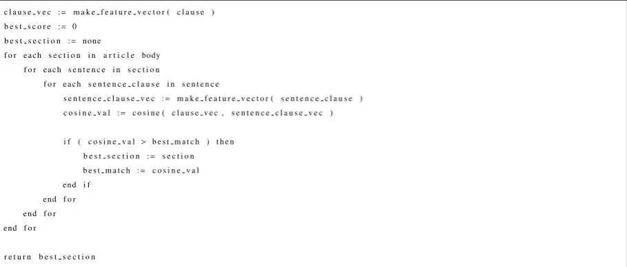
3.8.2 Clause Section Classifier . . . 34
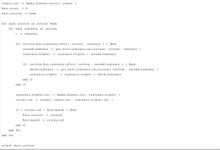
3.8.3 Clause-Triplet Classifier . . . 35
3.8.4 Sentence-Triplet Clause Classifier . . . 35
3.8.5 Section-Blob Classifier . . . 36
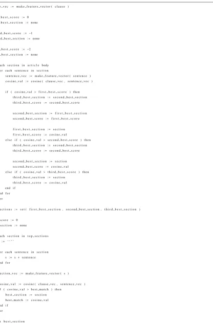
3.8.6 Bottom-Up Classifier . . . 38
3.9 Evaluation of the Proposed Methods . . . 39
3.9.1 Overview . . . 39
3.9.2 True Positives, False Positives, & False Negative . . . 39
3.9.3 Precision . . . 40
3.9.4 Recall . . . 40
3.9.5 F1Score . . . 40
4.1 Overview . . . 42
4.2 Performance Calculation . . . 43
4.2.1 Feature-Vector Creation . . . 43
4.2.2 Classification Procedure . . . 43
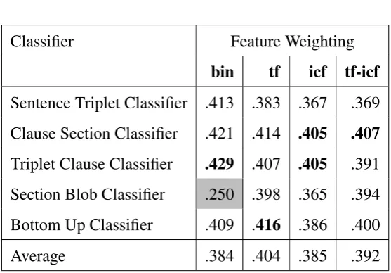
4.3 Feature-Weighting . . . 44
4.3.1 Motivation . . . 44
4.3.2 Feature-Weighting . . . 45
4.3.3 Results . . . 45
4.3.4 Conclusion . . . 47
4.4 Feature-Set . . . 48
4.4.1 Motivation . . . 48
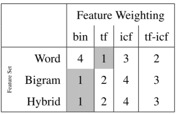
4.4.2 Overall . . . 49
4.4.3 Breakdown by Classifier . . . 52
4.4.4 Conclusion . . . 54
4.5 Filters . . . 57
4.5.1 Motivation . . . 57
4.5.2 Results . . . 57
4.5.3 Conclusion . . . 62
4.6 Fixed-Expressions . . . 64
4.6.1 Motivation . . . 64
4.6.2 Results . . . 65
4.6.3 Conclusion . . . 66
4.7 Classifiers . . . 66
4.7.1 Motivation . . . 66
4.7.2 Results . . . 67
Clause-Section Classifier . . . 67
Clause-Triplet Classifier . . . 68
Bottom-Up Classifier . . . 72
Conclusions . . . 74
5 Thesis Conclusions 78 5.1 Conclusions of Our Work . . . 78
5.1.1 Feature Weighting . . . 78
5.1.2 Feature-Set . . . 78
5.1.3 Filters . . . 79
5.1.4 Fixed Expressions . . . 79
5.1.5 Classifiers . . . 80
5.2 Overall Conclusions . . . 82
5.3 Applications of Our Work . . . 83
5.3.1 Proving Ground for Pre-processing . . . 83
5.3.2 Classification as a Feature . . . 83
5.4 Future Work . . . 84
5.4.1 Evaluation Towards Goal . . . 84
5.5 Ensemble Classification . . . 85
5.6 Other Domains . . . 85
6 Glossary 86
7 Stop Words 88
8 Bibliography 90
Curriculum Vitae 94
3.1 Most frequent corpus bigrams . . . 30
3.2 Clause Section Classifier . . . 35
3.3 Clause-Triplet Classifier . . . 36
3.4 Sentence-Triplet Clause Classifier . . . 37
3.5 Section-Blob Classifier . . . 38
3.6 Bottom-Up Classifier . . . 41
3.1 Corpus size reduction by filters . . . 15
3.2 Lemmatization mapping . . . 26
3.3 Percentage of bigrams containing each part-of-speech . . . 31
4.1 Scores with Word Feature Set . . . 45
4.2 Average score for each feature-set & feature-weight pairings . . . 49
4.3 Relative ranking for each feature-set & feature-weight pairings . . . 49
4.4 Scores for each feature-set, feature-weighing, and classifier configuration. . . . 51
4.5 Improvements from alternate feature-sets. . . 53
4.6 Rankings for feature-weighting, feature-set, and classifier configurations by feature-set. . . 53
4.7 Rankings for feature-weightings, feature-sets, and classifier configurations by feature-weighting. . . 55
4.8 Relative rank across feature-weightings per classifier/feature-set pairing. . . 56
4.9 Relative ranking of filters . . . 58
4.10 Filter/classifier pairings with the binary feature-weighting. . . 59
4.11 Filter/classifier pairings with the term-frequency feature-weighting. . . 60
4.12 Filter/classifier pairings with the inverse-corpus-frequency feature-weighting. . 61
4.13 Scores for all configurations of feature-weightings, filters, and classifiers. . . . 63
4.14 Fixed-expression filtering with bigram feature-set. . . 76
4.15 Fixed-expression filtering with word feature-set. . . 77
Introduction
The project began following an extended discussion with Professor Pete Rogan from the
Department of Biochemistry at The University of Western Ontario and President of
Cytog-nomix Inc. CytogCytog-nomix sells DNA probes for the purpose of confirming the presence, or
absence of a gene, corresponding to the given probe in a sample. These probes can be used by
cytogeneticists and genetic counsellors for diagnosing congenital conditions. Often, a genetic
counsellor will take note of a patient’s phenotypes, postulate an underlying genetic condition,
and then order probes to test an acquired genetic sample for the condition.
Professor Rogan was interested in a system that could mine a biomedical corpus and match
phenotypes to conditions and these conditions to specific genetic mutations. He also desired
that such a system would be able to handle contradictory claims by assessing the relative merit
of each claim using context: repetition of the claim within the corpus, agreement with the rest
of the corpus, citations counts, the impact factor of the journal, and the publishing history of
the authors. It was hoped that this system would allow genetic counsellors to input the patient’s
phenotypes and the system would, upon additional consideration of the incidence rate of any
relevant conditions, determine in which order probes should be tested to optimize reaching a
diagnosis.
While it was clear that such a system was beyond the means of our project, we attempt
to solve one of the components necessary for such as system: focusing on identifying and
extracting the main claims of biomedical research articles. Dr Barbara White completed her
PhD at The University of Western Ontario on inter-annotator agreement of human annotators
coding claims in biomedical journal publications [1]. She had been hoping to receive a grant
to further her work by enlarging her corpus, and we had been hoping to use her corpus both
as our own and as a gold standard for our work on claim extraction. Unfortunately, she was
not able to continue her work on her corpus, and we judged its current state insufficient for our
needs.
Furthermore, we hoped that we could compensate for the lack of a sufficiently large
an-notated corpus by using what we called the “greatest hits” model of abstract writing. It was
our belief, at the time, that the sentences in the abstract were sourced from the most important
sentences in the journal article’s argumentation. By matching each sentence from the abstract
with a sentence in the body of the article, we would then uncover loci of the most important
argumentation in the article and be able to extract the main claims from them. Additionally, we
believed that our biggest challenge would be accounting for changes in tense, pronoun
replace-ment, etcetera that had been made for reasons of grammar and conciseness to the sentence as
it had been copied from the body to abstract.
This approach, however, was discouraged when we met with a subject matter expert, Dr
Derek McLaughlin, who instructs undergraduate students in the biomedical field in
profes-sional writing for the sciences. He informed us that the lifting of entire sentences from the
article body was considered a bad practice, and, if anything, we should look for similarities at
the clause level rather than the sentence level, due to the compressed nature of an abstract.
Our discussion with Dr McLaughlin left us wondering how to establish a corpus. We then
looked into the MEDLINE collection of journals, since they often have a structured abstract. A
structured abstract is one where the abstract is organized into the same sections as the sections
which appear in the body of the article. We realized that these journal articles with their
structured abstracts could serve as an annotated corpus. MEDLINE also had the advantage
of being online and being stored in an XML format.
article body for the purpose of the establishing loci of argumentation ripe for extracting, we
came to see it as a problem that could be approached in three separate stages. The first is
selecting the corresponding section for each sentence in the abstract; the second is sub-selecting
from that section a specific sentence to match the one from the abstract; and third is mining the
matched sentence’s loci for claims. By using the structured abstracts as an annotated corpus,
we felt we could meaningfully investigate the first stage of the problem. However, following
Dr McLaughlin’s advice, we decided to focus on matching clauses from the abstract instead of
sentences.
1.1
Research Question
Since our approach is novel to the field, our work, by definition, had to be exploratory; thus,
we have no pestablished performance goals or results to which to directly compare our
re-sults. Our research is driven by the following question: how can we maximize the performance
of using word similarity to label clauses in abstracts to their referent article body sections?
We implemented several different classifiers that use the cosine measure of similarity and
ap-plied various techniques to them that have been used in other natural language processing or
classification tasks attempting to improve the heuristics’ performance.
1.2
Approach
Our approach was to try out various techniques and to be experimental and exploratory. In
our search of the literature, we did not find any related work which could serve as a benchmark
for our own work. Thus, we felt, for this approach to be fruitful in the long term, it would be
up to us to establish a baseline for further work by others to improve upon. To this end, we
applied various techniques that have been known to be efficacious in both the fields of artificial
intelligence and natural language processing research, and we measured their effect on our
underlying and unquestioned assumption was that anything that improved our classifiers would
ultimately improve the ability to assign the clauses from the abstract to specific sections of text.
1.3
Organization
This thesis, like our corpus, is organized following the conventional IMRaD structure: an
Introduction, followed by a Literature Review, and then Methods, Results, and Discussion
sections. The Introduction consists of the backstory that led us from the original inspiration for
our research to the final research question upon which we settled, then a clear statement of our
final research question.
The Literature Review examines the published work that most closely resembles our own.
The work is generalized along the lines of the corpora other researchers used, their
methodolo-gies and the features they used for their own classification. Following that is an examination of
how our work is both an extension of the field and a novel outgrowth of it.
The Methods chapter starts with a discussion of the composition of our corpus along with
statistics concerning word frequency. Then, we define and describe our motivation and
proce-dures for our five experimental variables: feature weighting, feature-sets, text pre-processing,
and classification heuristics.
The Results chapter begins with an overview of the section and then reviews the results
of the experimental variables in the order in which they are presented in the Methods section.
Each method is evaluated fully. For all but the final experimental variable (the classifiers), each
variable is explored full, but only select configurations are carried forward to be used as the
basis for the exploration of the next experimental variable. However, for the classifiers, there
is a full review of how each classifier performs with each other experimental variable.
Finally, this thesis ends with a Conclusion chapter. This section states the conclusions that
can be drawn from our work. It also suggests steps to both further our work and how to apply
Literature Review
2.1
Corpus Construction
There has been a tremendous growth occurring in the amount of research being performed
in the biomedical disciplines, and this increase has lead to a large volume of high-quality
research articles being published in journals. As happens with such an influx of material,
dif-fusing this information has become an issue. For this reason, research articles from biomedical
journals often form the corpora of natural language processing research [2-14]. Specifically,
in the literature, there is a focus on randomized control trials [7,12,15,16]. Fittingly, the other
major discipline whose research is found in corpora is computational linguistics. This is most
likely because the researchers are better able to assess the material with which they working,
especially when manually annotating it [17]. This is important because, as discussed below,
access to subject-matter experts is an issue which restricts the size of corpora available for
analysis.
In the literature, there are roughly three sizes of corpora, and the size of the corpus is
generally a function of the methodology and tooling used. Whenever the research methodology
incorporates manual annotation as a part of the methodology, the corpus sizes range from
6 to 20 articles [9,10,13,17]. When the corpus is processed solely by researcher-developed
tools, the corpus sizes are generally in the hundreds of articles [3,14,15,18]. It is only when
research leverages pre-existing tools, such as search engines, do the corpora grow to thousands
of journal articles [13,16], even up to including the entire PubMed corpus.
According to Liakata et al., “abstracts of much high-quality work remain unstructured”
[16]; however, many researchers focus on structured abstracts, using the structure as additional
information. Some use structured abstracts as labelled training data [4], and others use journal
articles with structured abstracts for its corpus exclusively [6,12,15,16]. Demner-Fushman and
Lin leverage MeSH (“Medical Subject Headings”) headings [16] that are applied by trained
annotators [19].
While MeSH tags are generated by hundreds of trained annotators, those annotators are
not employed as part of any specific research project but rather directly for PubMed itself, and
no individual research project employs nearly as many annotators [19]. Nigam et al. utilize
data that is labelled into the classes that research is classifying [20]. Other data [4,9,10,15,18]
are annotated by only one annotator and some with expert guidance [4,18]. While Yamamoto
and Takagi’s corpus has 202 manually labelled articles [4], only the abstracts are annotated
(1652 sentences). While the corpus in Mullen et al.’s work annotated entire articles [10], it
only has 20 articles. Wilbur et al.’s work had 12 annotators [11]: the three article authors and
nine graduate students in the sciences; however, they only annotated 101 sentences. From 148
RADIUM-structured journal articles, Agarwal and Yu chose 5 sentences from each section
for 2960 sentences [6], 2000 of which were annotated by the article author and one of five
biomedical researchers. Shatkay et al. had eight well-trained annotators [13], and while each
sentence was annotated by three different annotators, they annotated only 10,000 sentences.
The largest corpus is Liakata et al.’s work [14], which had 20 annotators who were a mix of
chemistry PhD s and post-doctoral students, and yet they annotated only 265 articles. This
2.2
Methodology
In the literature reviewed, the most commonly used metrics for benchmarking are the F1
-score and the kappa--score. Generally, the F1-score is used to measure classifiers classifying
previously manually annotated data, whereas the kappa-score is used to measure the ability of
independent annotators to reach the same conclusion with regards to annotating a given piece
of text:
Fβ =(1+β2)· β2precision·precision·recall+recallF1= 2·
precision·recall precision+recall
The F1-score is used with classification tasks as a combined measure of a classifier’s
pre-cision and recall. It is calculated by comparing the classification output of the classifier with
the independently determined “gold standard” classification. This gold standard is presumed to
be completely accurate and is generally established beforehand. Precision is the percentage of
classifications that are correct, whereas recall is defined as the percent of available
classifica-tions actually made by the classifier. By default, an equal weighting is given to both precision
and recall, but by tuning theβ-parameter, the score can be adjusted to place greater emphasis
on either statistic [12,15,18]; in fact, McKnight and Srinivasan explicitly state that they use 1
as the value for theβ-parameter [12].
κ= Pr(a)−Pr(e) 1−Pr(e)
The kappa score is the difference between observed classifications and what one would
expect by random chance. It is used when there are multiple independent annotators annotating
a given corpus. Their annotations are then compared to one another’s, and their inter-annotator
agreement is measured. It is important to note what distinguishes the kappa-score from the
F1-score. The F1-score requires a definitive annotated copy against which the other annotated
copies are compared, and the kappa-score does not. The kappa-score treats each annotated
copy as equal and presumes that, a priori, there is no reason to prefer one annotated copy over
another. Thus, it is used when analyzing the reproducibility of an annotation scheme [6,17].
The most common method for classifying text is through the use of machine learning with
approaches in support vector machines (SVM), conditional random fields (CRF), and Naive
along with Liakata et al. started with linear kernel [4, 14], but Yamamoto and Takagi switched
to using polynomial kernel [4]. The Naive Bayes classifier is a well-studied and widely-used
classifier based on observed conditional probability [21]. From the training data, the
probabil-ity of each classification in the presence of feature is observed (i.e. calculated). Then, when
classifying, the presence or absence of each feature is determined, and the overall probability
is calculated for each class. Finally, the one with the highest probability is selected.
Mizuta et al. and Teufel et al. [10,17], in attempting to maximize reproducibility,
struc-ture their annotation guidelines as decision trees. This approach is generally seen when the
annotation is being performed by humans. Nigam et al. uses a statistical technique called
“maximum entropy” [20]. The key assumption is that in the absence of additional information,
one should presuppose a uniform distribution of classes. Then, additional facts are observed,
such as when feature A is present, the class is Z 40% of the time, and the other 60% of the time,
the classification is spread uniformly amongst the remaining classes. In the absence of feature
A, a uniform distribution amongst all the classes is once again the case. Chung uses a similar
technique called “Conditional Random Fields” [15]. Both maximum entropy and conditional
random fields can be generalized together as different forms of “log-linear models” [22].
As is common with many machine-learning tasks, most projects [6,9,12,13,18] use k-fold
cross-validation. Nearly all of the projects use 10-fold cross-validation [6,9,12,18] with a
project [15] using more (fifteen) and another [13] using less (five). McKnight and Srinivasan
state that they randomly split the data into folds [13]. Agarwal and Yu randomly split the data
into folds of random sizes between 100 and 1,000 in increments of a 1,000 [6].
In the reviewed works, little emphasis is placed on pre-processing of input documents.
Nigam et al. explicitly state that they do not filter stop-words or use stemming [20]. In Agarwal
and Yu [6], they replaced all numbers with the special token “#NuMBeR” which is unlikely to
occur in the source text. Chung tried a variation of the approach where researchers replace all
numbers with either “INT” or “REAL”, depending on whether the number in the source text
represents an integer or real number value [15], where others replace citations with the token
An open question in the literature is the size of the unit of text used for annotation: should
annotation occur at the sentence or clause-level? Liakata et al. admit that there is “no general
consensus” [14]. Mizuta et al. choose to annotate at the clause-level [10], and Mullen et al. do
both [9]. Wilbur et al. [11], by contrast, choose to annotate at the sentence level while allowing
annotators to, at their own discretion, annotate at the clause level. This later causes problems
when comparing annotations between annotators when the units do not match up. No reviewed
research articles propose a unit of annotation larger than the sentence (e.g. such as paragraph)
nor smaller than the clause (for example, the word or noun-phrase level).
2.3
Features
Within the domain of using natural language processing to classifying text in
biomedi-cal journal articles with regards to rhetoribiomedi-cal status, most of the work reviewed does not use
decision trees for their classification (however, Mizuta et al. do [10]) but instead use
machine-learning. Thus, it is of the utmost importance that careful attention is paid to the selection
of features used. Unsurprisingly, the features are generally derived from the words in the text.
Generally, most of the reviewed literature uses what is called a “bag-of-words” approach where
the focus is on the word tokens present, with little to no leveraging of the grammatical or the
rhetorical structure of the document or other higher-level concepts (the use of sequences of ‘n’
words, called n-grams, is still considered a bag-of-words). Only one study truly veers from the
model using cue phrases, syntactic structures, and word order [7].
Like most of the other articles, Shatkay et al. [13] use individual words as features, but
they augment the individual word features with additional features from both the bag-of-words
approach and features, which leverage deeper syntactic information. From the bag-of-words
approach, they use both bi- & tri- grams, which they call “statistical phrases” and leverage
deeper syntactical structure with noun- and verb- phrases, which they refer to as “syntactic
phrases.”
augment it with bi-grams, using only features whose frequency is greater than three. Liakata et
al. [14] have some other local features such as the presence of citations, sentence length, verb
parts of speech, passive voice, grammatical subjects, and grammatical structures.
Without a doubt, the most consistently relied upon feature in the literature is the presence of
words in the text fragments. While some researchers do incorporate a part-of-speech alongside
the textual representation of a word, the words are treated, regardless of their part-of-speech,
as if the part-of-speech was just part of the word token itself, and all parts-of-speech are treated
uniformly. However, some researchers treat certain parts-of-speech differently. The main thrust
of this has been focusing on the role that verbs play as seen in varying degrees [4,7,10,11,14].
Some researchers [7,10,11], specifically focus on verb tense; for example, Wilbur et al. find
that the usage of “were” usually precedes the exposition of a finding [11]. Outside of verb
tense, no other single aspect of verbs is studied as broadly. Yamamoto and Takagi examine for
the presence of an auxiliary verb [4], Mizuta et al. the main verb [10], de Waard the modality
of verbs [7], and Liakata et al. the passive voice [14].
After words, the most widely used feature in the literature is bi-grams. The bi-grams do
not have to be directly extracted from the corpus; for example, Mullen et al. lemmatize them
first [9]. Some [9,13,14] only use the bi-grams whose frequency crosses a given threshold.
McKnight and Srinivasan do not use bi-grams but mention that they plan to do so in their
future work [12]. Shatkay et al. do include some tri-grams [13], but their prevalence in the
literature is significantly less than that of bi-grams.
An important non-word based feature that reoccurs in the literature is that of the position of
the text fragment relative to the document. This is found in one degree or another in much of
the research [4,6,9,12,14,15,18]. As in Yamamoto and Takagi [4] or McKnight and Srinivasan
[12], the measurement is often represented as a percentage in the range of 0 to 1, where 0 is
the very first sentence, and 1 is the very last. Liakata et al. use both the position of a sentence
within a paragraph and within a section [14].
Despite bag-of-words being the predominant approach used in the literature reviewed,
“windowing.” Windowing is a technique in which, when classifying a piece of text,
infor-mation derived from surrounding text is considered. For example, Agarwal and Yu use an
estimated tag for the preceding sentence as a feature for classifying a sentence [6]. Kim et al.
do that as well [18], but it also simply reuses features from previous sentences like Chung does
[15].
Most of the articles reviewed used feature-vectors either directly (e.g. with a cosine
mea-sure) or as input into machine-learning algorithms. In either situation, how to represent the
various features numerically poses a challenge: specifically, how does one quantify the
pres-ence of words and bi-grams in a text sample? Shatkay et al. [2] use simple binary values to
indicate the presence or absence of a feature. Nigam et al. [20] use the term frequency in their
vectors. Yamamoto and Takagi [4] use the term frequency in the sample relative to the term
frequency in the corpus (i.e. term-frequency-inverse-document-frequency). McKnight and
Srinivasan initially try multiple schemes [12], but “all performed similarly,” so the researchers
chose a binary representation.
2.4
Comparison to Field
Our research methodology clearly follows the groundwork established by others in the field.
Like many others, we use biomedical publications from PubMed with structured abstracts. The
size of our corpus (which is approximately 100 articles) corresponds with what is generally
seen when the corpus is processed programmatically (i.e. without human intervention) but
while not leveraging external resources such as the MedLine search engine, MeSH tags, or
UMLS (“Unified Medical Language System”)[23]. Our evaluation methodology uses the F1
-measure present in nearly all of journal articles in the field surveyed. The use of pre-processing,
which we heavily employ, is seen in the literature, but not as commonly as one might expect.
While the features, words, and bi-grams we employ are nearly universally used, the cosine
measure is not. It does see some usage in the literature [3]; however, as most research heavily
cosine measure-could be used as a feature for machine learning, as the values that went into
the cosine-measure are already present, the value is questionable when one has much richer
information already available for classification.
2.5
Contrast to Field
While, like the literature, our work does incorporate the F1-measure, we, unlike many, do
not calculate the kappa statistic. In the literature, the kappa statistic is applied to determine
agreement on the annotations made between annotators, but we do not employ any manual
annotation. If we considered each of our heuristics as an annotator, then we could calculate
a kappa-score for the clause-level agreement between heuristics, but it is not certain that the
measure would be indicative of the information we wish to pursue. This is not entirely
unprece-dented: our approach is supported since the kappa is not used in any of the machine-learning
approaches reviewed. However, while our approach has a passing resemblance to machine
learning (as least when contrasted with decision trees and manual annotation), it is a purely
sta-tistical technique. Over-fitting is principally a concern of machine-learning-based approaches,
which our approach is not; thus, we do not perform cross-validation because we are concerned
with over-fitting. Also, fairly notably, we do not exploit text-position as a feature: the abstracts
that we use are structured, and the article body sections appear in a fixed order. The clause
position would correlate too highly for the classes into which we are classifying for the clause
position to be useful for us as a feature, and it would hamper generalizability.
2.6
Value Proposition
Our work contributes to the body of knowledge in the field chiefly in four ways: it
supple-ments an existing body of knowledge regarding the processing of natural language in
biomedi-cal journal articles; we place a high emphasis on pre-processing, and our results are applicable
sourcing the referent section of clauses from abstracts, and our work can be used to augment
existing work; finally, our work establishes a platform for enabling annotator-less research into
biomedical processing.
Both the biomedical field, and the resulting field of the processing of its articles, are
increas-ingly active areas of research. As such, anything that explores this field, especially in a novel
way, is a welcome addition to the knowledge base. Our work presents a host of techniques that
can be grafted onto existing approaches. Unlike a lot of other work in this domain, our work
is focused solely on leveraging lexical similarity. The techniques we apply are those whose
intent is only to lay bare lexical similarity that may have been occluded by grammatical
neces-sity. Therefore, we do not attempt to leverage domain-specific resources and pre-existing tools
such as UMLS or MeSH tags, etc. As such, our techniques are applicable outside the domain
in which we are working. This will be increasingly important as more and more researchers
start branching out beyond the present biomedical niche into other fields.
Abstracts are believed to be the distilled points of argumentation of an academic article.
Therefore, there is hope that clauses from abstracts could be leveraged to indicate which areas
of a research article may be the most important (i.e. important enough that the writers felt
in-clined to include them in the abstract) for further information extraction. Labelling the referent
section is a proxy-goal that works in this direction.
One of the persistent problems within most sub-fields of natural language processing is that
of finding sufficient annotated materials with which to work. It usually becomes a trade-off
between the size, the accuracy, and the cost of establishing the corpus. As such, most research
is done on small corpora. Our approach is annotator-free and allows for other researchers to
Methodology
3.1
Introduction
We have found no references in the literature to anyone doing comparable work. As such,
there is no previous research which has established techniques that are known to work.
There-fore, we have selected a combination of techniques that are either known in the field of natural
language processing, suggested through discussions with subject matter experts, or created by
our own intuition. Thus, we consider our work to be exploratory and to suggest techniques for
use by others in the future.
3.2
Corpus Composition
3.2.1
Overview
Our final corpus consists of 92 biomedical journal articles, as some articles produced errors
when parsed with the chosen tools. There are a total of 29,186 sentences composed of 45,778
clauses, with a total of 594,236 words. The most frequently appearing word is “the”, and it
ap-pears 29,300 times. The most common part-of-speech in the top 100 words is IN (“preposition
Filter Words in Corpus Corpus Size Reduction
NullFilter 36,341
LowerCaseFilter 32,321 4,020
PoSFilter 32,832 3,509
PoSLemmatisationFilter 35,269 1,072
PunctuationFilter 36,336 5
StemmerFilter 35,023 1,318
StopWordFilter 36,092 24
SymbolFilter 36,328 13
POS JUNK 28,516 7,825
ALL 26,153 10,188
Table 3.1: The number of unique words in the corpus depends on the filter being used.
or subordinating conjunction”), but the part-of-speech that makes up the most of the corpus is
NN (“noun, singular or mass”).
Of course, the choice of filter affects the number of unique words in the corpus and varies
with the filter used in the configuration (see table 3.1 ). The choice of filter can reduce the
number of words in the corpus by nearly 30%.
3.2.2
Hapax Legomena
Of the over half-million words in the corpus, 36,341 of them are distinct (using the
case-sensitive string composition and part-of-speech definition). Nearly half of them (48%; 17,391
words) appear only once. Words that appear only once are called hapax legomena.
Surpris-ingly, only 5.3% of them are numbers. As the natural sciences involve many precise
measure-ments, one would expect that would result in specific numbers that are very large and very small
numbers that appear only once. Nouns combined compose over 64% of the hapax legomena
(NN, singular nouns alone were 54%), with all verbs combined (i.e. VB, VBD, VBG, VBN,
2.47% of the hapax, which means that the ratio of hapax legomena adverbs to verbs (16:64) is
similar to that of adjectives to nouns (19:64).
Of the distinct nouns (i.e. NN, NNS, NNP, NNPS), half of them are hapax legomena; by
contrast, only 37% of distinct verbs (i.e. VB, VBD, VBP, VBZ) are. The hapax legomena
represent 5.4% of the nouns but only 2.4% of verbs. It is not unexpected for there to be a
greater variety in nouns than in verbs, as scientific discourse requires naming very specific
items.
3.2.3
Word Frequencies
On average, each word in the corpus appears 15 times; however, due to the number of
hapax legomena, on average, a word that appears more than once will appear 28 times. This
high frequency is also deceptive because some parts-of-speech have very few words, but those
words have very high frequencies. Such a class is TO (which represents both the preposition
and infinitive marker “to”), which contains only two words but represents a total of 9,583 words
from the corpus. When one looks at the average frequency of words that are not hapax legomen
and do not belong to a high-frequency part-of-speech (i.e. average frequency>100; there were
13 such parts of speech none of which were parts expected to convey important context), that
number is 19 appearances.
The ratio of adjectives to nouns is fairly similar, whether or not one looks at unique words
or total number of words (30% and 28% respectively). This also holds true for the ratio of
adverbs to verbs (23% and 24% respectively). The fact that they behave similarly is interesting
because adjectives are only 18% of the unique words and 10% of the total, and adverbs are
only 2%. Despite there only being 37 distinct words classified as determiners (i.e. DT), they
make up close to ten-percent (9.49%) of the total words.
The average noun appears 9.3 times in the corpus. Nouns of the most common class of
nouns (i.e. NN, “singular or mass”) appear on average less, at only 8.4 times, whereas the
3.2.4
Top 100 Words
In the corpus, the most common word is “the”, followed by “of”, and then the period (“.”),
the comma (“,”), and then “and”. The words with the IN part-of-speech make up 16% of the
top 100 most frequent words, but their combined frequency makes up 30% of the combined
frequency of the top 100. Words with NN part-of-speech (i.e. singular or mass nouns) comprise
15% of the words in the top 100, but their combined frequency is just under 5%. DT make up
11% of the top 100 and 19% of the combined frequency. There seems to be no correlation
between the distribution of frequencies across the top 100 words and across the entire corpus.
Of the top 20 most frequent words in the corpus, all of them are either stop-words or
punctuation. “Stop-words [are] common words such as ’the’ or ’and,’ which help build ideas
but do not carry any significance themselves” [24]. Of the top 40 most frequent words, only
7 are content; extending to the top 50 words, the number of content words only rises to 11.
The first “content” word is the 23rd most frequently appearing in the corpus: it is the plural
noun “cells.” This is interesting because there are many more singular nouns than plural nouns
in the corpus. The first singular noun is “protein” at 27th, followed by “genes”, which is
31st. The word “cell” is very close in the frequency ranking to “cells” (36th and 23rd overall,
respectively). If they were counted as one word, their frequencies combined (1310 and 2111)
would make cell/cells the 16th most frequent word. This finding reinforces the notion that
stemming and/or the inverse-corpus-frequency feature-weighting are worth exploring.
Although stop-words dominate the higher end of the word frequency spectrum, they do
not span the entire gamut. The stop-word “got” appears at the very bottom with only one
appearance in the entire corpus. This is somewhat surprising as one may have expected all of
the stop-words to appear frequently.
Nouns have a lot more repetition than verbs. The most frequent non-stop verb is “using”,
33rd overall, followed by “used”, which is 56th. The 76th is “shown”. The most common
verbs all tend to be different forms of “to be” (i.e. “is”, “were”, “was”, “are”, “be”, “been”),
followed by verbs related to the IMRAD (“Introduction, Methodology, Results, and
“observed”, “described”). In fact, if one combines that category of words (i.e. “shown”,
scribed”, “found”, “observed”, “compared”, “reported”, “shows”, “show”, “suggest”, and
“de-termine”), then it would be the 20th most frequent word found in the corpus. The most frequent
biology-related verb is 215th overall (“expressed”, as related to the concept of “gene
expres-sion” with a frequency of 253rd), and the next one is “treated”, 255th overall, appearing only
227 times. This information regarding the frequencies of nouns and verbs suggests that nouns
are much more likely to reflect the domain than the verbs. However, the research does not
consider weighting different parts of speech.
3.2.5
Distribution Curve
The most common word in the corpus is “the”, and it appears 29,300 times, even more
times than “.”, constituting an entire 5% of the corpus. Considering that there is a total of
36,341 distinct words in the corpus, that means for every distinct word in the corpus, “the”
appears 0.8 times. The lowest recorded frequency is, not unexpectedly, 1, and there are 17,391
words with that frequency. Thus, the most frequent word appears more times than the number
of words in the corpus that appear only once; “the” actually appears 1.7 times more than the
number of hapax legomena.
The composition of our corpus is arguably atypical. While the three most frequent words in
our corpus (ignoring the period and the comma, which are not considered words in the Brown
corpus [25]) are the same (i.e. “the”, “of”, and “and”) and in the same order, and the following
three (i.e. “to”, “a”, and “in”) are not, the rest of the list is noticeably different. The frequency
distribution is also quite different. “The” represents only 5% of our corpus instead of 7% as in
the Brown corpus [25,26]. Furthermore, our corpus also does not follow Zipf’s law. Whereas
Zipf’s law predicts that frequency of works in the corpus is inversely proportional to the rank,
in our corpus frequency decays exponentially with rank. In the Brown corpus, the 135 most
frequent make up half the corpus, in ours it is the top 153 [27]. What causes our corpus to be
different was not investigated in this study, but it could be due to the subject matter and/or our
Half of the corpus is made up of 36,118 distinct words with a frequency of 284 or less; the
other half is made of the top 186 words. The top 3 words make up nearly 10% of the corpus;
nearly a quarter of the corpus is made up of the top 8 most frequent words. On the other end
of the spectrum, words with a frequency of 7 or less (representing 29,603 distinct words) make
up nearly 10% of the corpus. For a quarter of the corpus, one needs only 34,655 distinct words
that appear 44 or less times in the corpus.
In the corpus, there is at least one word with a frequency for every number between 1 and
142; for numbers equal to or greater than 699, if there are words with that frequency, there is
only one such word. Only 5 frequencies greater than 368 have 2 words or more words.
3.2.6
Sentence Lengths
The sentences in our corpus range in length from one to a hundred words long. The average
sentence is 20 words long, the median is 18.5 words, and the mode is 16 words. Nearly,
without exception, as the absolute value of a sentence length from 16 increases, the frequency
decreases. The notable exceptions are an uptick when going from sentences of length two to
length one and amongst the last 16 sentence lengths (i.e. 66-100) where the frequencies are in
the low single-digits.
It is important to remember that the corpus was not tagged by hand but rather using PostMed.
As such, one would expect oddities in the data from the use of classifiers. While it is possible
to form a complete sentence with only a single word—“Stop!” is a complete sentence—our
corpus contains 532 one-word sentences; most of these are titles and errors in determining
sen-tence boundaries. One such problem is when periods are not used to end a sensen-tence but rather
to indicate an abbreviation such as “Dr.”. Likewise, there is a sentence in the corpus that is 100
3.3
Processing Pipeline
When processing the corpus it is done in the following steps. First, each paper is processed
with StepByStep, a derivative of the STEPS2 framework. This extracts the article content from
the .nxml files, tags the words according to their part of speech, and then the sentences are
parsed using the Collins parser. The parsed sentences are then read in line by line where a
graph representing the parse tree structure is constructed. Any input filtering is applied at this
time.
When creating the words, as per our definition, a fly-weight pattern (via a factory pattern) is
used so that the words themselves are “instance controlled”. This means that only one instance
of every word will exist. By using a factory pattern we can also easily keep track of the usage
of the word in the corpus (i.e. the “corpus frequency” ). When we are doing fixed expression
filtering then we perform this phase twice; first, to identify the fixed expressions from the text,
and again to replace the fixed expressions. We reset the word counts after the initial pass as not
to distort the frequency counts for words replaced by the fixed expressions.
To perform the classification we iterate through the clauses in the abstract, creating a feature
vector for each one. Then, for each clause, we iterate through the rest of the document in a
manner specific to the classifier’s implementation. Feature vector values are modified by the
feature weightings as they are created.
Once the classifier has finished processing the document, the classifier returns it’s
classi-fication. This is compared with the section of the structured abstract from which the clause
was taken. If the classification is correct it is considered a “true positive” for the expected
article body section type (e.g. ‘results’), for the purposes of the F1 measure. Otherwise, it is
counted as a “false positive” for the article body section returned by the classifier, and a “false
negative” for the known section. The F1 measure is calculated for each article body section
and their scores are combined into an arithmetic average weighted by the expected numbers of
3.4
Feature Weighting
The use of a cosine measure to gauge similarity between text fragments was part of our
initial experimental design. However, when the implementation of the cosine measure began, it
became apparent that a variety of implementations of the cosine calculation are in fact possible.
The basic idea of each value corresponding to a feature of that text fragment (presence or
absence of a word from the corpus in our case) remains constant. However, it occurred to us
that using such a method implies (by resulting in the same score for the measure) that two text
fragments sharing just the word “the” are equally as similar in content and intention as two text
fragments sharing the word “haemoglobin”. In other words, the cosine measure considers both
sets of text fragments as being equally similar even though “the” is considered a stop-word and
“haemoglobin” is a much rarer word whose appearance is generally restricted to the biomedical
domain.
Upon realizing this deficiency, the first approach involves sub-selecting words (such as
stop-words) that would not count towards the feature vector. While this approach inspired the
filter experimental variable, it is problematic. Even if a certain class of words (such as
stop-words) is ignored, there remain issues with other classes of words. For example, should we
consider text fragments just sharing the word “blood” (just over a trillion results in Google)
to be judged as similar in content as two fragments just sharing the word “haemoglobin”? We
felt the answer to that was “no” but also that two fragments just sharing “blood” should be
scored as being more similar in content and intent than two fragments just sharing the word
“the”. It became apparent that the logical conclusion results not in two categories of words
but rather a near infinite hierarchy of categories of words and that categories could be defined
by their repetition within the corpus (i.e. corpus frequency). The generalization became then
that text fragments sharing rare words should be judged as being more likely to have the same
intent as fragments sharing more mundane words. Thus, the question was formed: can we get
higher performance if we weight features (i.e. words) by their rarity (specifically, by the inverse
frequency in the corpus) when creating feature vectors representing those fragments? We then
times is indicative of both having the same intent (i.e. term frequency).
3.5
Feature-Set
Our features are represented within our system by the means of a “feature vector”—an
array of measurements where each position within the array corresponds consistently with a
feature. Therefore, by comparing values at the same index from multiple feature vectors, one
can compare how they vary along the corresponding measure [28]. We compare our feature
vectors by computing their dot-product, which is the measure of the cosine between the two
vectors. When the feature vectors are identical, the value of their cosine is 1. When the feature
vectors are entirely dissimilar (i.e. orthogonal, not negated), the cosine will be 0 [28].
The purpose of feature-vector cosines is to use the measure of the similarity between the
feature vectors of two text fragments as a proxy for measuring the similarity of their semantic
intent, which guides us in matching the clauses from the abstract to sections from the article
body. The unstated assumption is that a similarity of words between text fragments is an
effective indicator of similarity. To explore this assumption, we compare the performance of
using the sharing of words —as a measure of overlap— to that of sharing bi-grams. To perform
this comparison, we replace the presence of words in the feature vectors with the presence of
bi-grams. A third option we explore is whether combining the feature-sets (that is appending a
bi-gram feature vector to a word feature vector) improves the performance.
So to restate our experiment, for the experimental variable of a feature-set, we have three
values: words, bi-grams, and the union of words and bi-grams (the hybrid feature-set).
3.5.1
Word Feature-Set
In the word feature-set, each position in the feature corresponds to the measure (e.g. 1
for presence or 0 for absence) of the word from the corpus corresponding with that location.
This is the most likely approach and is the one used in the preceding section exploring the
3.5.2
BiGram Feature-Set
The second value for this experimental variable is the usage of bi-grams. N-grams are
se-quences of tokens (whether the tokens are words, syllables, letters, etcetera depends on the
implementation, but here we are using words), which are often used in computational
linguis-tics. As the size of a text grows, the number of n-grams grows exponentially, especially for
larger values of N, most of which appear quite rarely. When the number of n-grams is very
large, their distribution is unlikely to be reflective of the texts of which the corpus is a sample.
Due to these limitations and the size of our corpus, we only use n-grams of size two, which are
usually called “bi-grams”; this is our second feature-set. N-grams of size 3, 4, and 5 have only
recently begun to be used by researchers at Google with a corpus that is one terabyte in size
and contains over a trillion words [29].
3.5.3
Hybrid Feature-Set
The third value for this experimental variable is a combination of the feature-sets. This is
done by coupling the word feature-set and the bi-gram feature-set. Each position in the feature
vector is still associated with only one element from the feature-set. This experimental variable
is important because even if one of the other two feature-sets has clearly superior performance
to the other, we know if the less performing feature-set can augment the other for increased
performance. When a feature-vector is constructed for a text-fragment, the feature-set reflects
the entire corpus and not just those features that are present in that article.
3.6
Filters
As stated earlier, our operative definition of a word is a part-of-speech and a case-sensitive
sequence of characters denoting the text token of the word. Two words are only considered
equal if both the text token and the part of speech are the same. Therefore, a word is only equal
to itself, even if the two words are so similar to readers that they would consider them
match between two words, but our classifiers will fail to. For this reason, we chose to explore
the effects of what we called “text filters”. The purpose of a text filter is to systematically
trans-form the incoming text, in a deterministic way, to remove differences between words which are
believed to be superficial and to expose to the classifiers to the similarity that appears to the
reader. By applying these filters to the text during input, they will allow the classifiers to make
some matches similar to that of a human reader. When filters are included in configuration,
words that have been processed by the filter are used in the matching process. The term “filter”
is borrowed, as a metaphor, from the colour filters that are sometimes used in photography.
It is our assumption that clauses in the abstract, those which refer to specific sections of
the body, would often have minor differences than the actual words with which they were
composed, to express their ideas to adjust for different tenses being used or to better fit the
surrounding text for flow. Other times, clauses in the abstract get rephrased for concision,
especially when multiple sentences are united (e.g. a word that would have been originally
capitalized at the beginning of a sentence no longer is).
When brainstorming, we established eight different filters: the null filter; the lower-case
filter; the part-of-speech filter; the part-of-speech lemmatization filter; the punctuation filter;
the Porter-stemmer filter [30]; the stop-word filter; and the symbol filter. A ninth, a meta-filter,
was created which could combine any number of other filters. For our research, we created two
such combinations of filters, which are discussed last after all other filters: the POS JUNK and
ALL FILTER (see table 3.1).
3.6.1
Individual Filters
Null Filter The null filter is the most basic filter. It does nothing to text but it returns the
unmodified word with both the original word token and the part-of-speech tag. It is used as the
default filter for a configuration when no filter is otherwise specified.
Lower-Case Filter The lower-case filter leaves the part-of-speech tag unchanged, but it
capitaliza-tion of the first letter of a word appearing at the beginning of a sentence is enough for it to be
considered a different word by our definition. Thus, even a simple reordering could prevent
what might seem like an obvious match. Consider the following two phrases: “Blood was
viscous” and “The blood was viscous.” Using our operative definition of word, they share only
two words: “was” and “viscous” but not “blood”/“Blood”. However, when the lower-case filter
is applied, there are three words shared by those text fragments. When this filter is applied, it
effectively removes the case-sensitivity criteria from our definition of equality between words,
since all words will be entirely lower-case. Employing this filter will then illustrate the effect
on performance that considering case-sensitivity has.
Part-of-Speech Filter The part-of-speech filter removes the part-of-speech from words so
that they are judged entirely on the basis of their text token. Removal of the part-of-speech tag
from words is implemented to reassign all words to have the same part-of-speech. This filter
provides a base against which the part-of-speech tag can be compared.
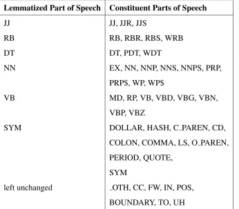
Part-of-Speech Lemmatization Filter The Collins-parser tags words to nearly 50 different
parts-of-speech categories. The part-of-speech lemmatization filter was designed to see if,
perhaps by merging existing categories, using fewer ones would improve performance. A
“lemma” is defined as “a set of lexical forms having the same stem, the same major part of
speech, and the same word-sense” [28]. This process is known in natural language processing
as “lemmatization”. This “merging” takes all the various parts-of-speech and breaks them into
distinct groups, where one member of the group is selected to be representative of that whole
group, and all words with tags in that group are retagged to have the part-of-speech that was
chosen as representative.
We have two distinct hypotheses for suggesting that filters aid classification. The first is that
with the size of our corpus, there may be too little repetition to accurately gauge the frequency
of words, and perhaps by merging categories, we can simulate the effects of a larger corpus.
Confirming that this filter approximates a larger corpus is out of the scope of this particular
The second is guided by the belief that clauses are often slightly modified from the form
they have in the article body when they are repeated in the abstract. These most common
modifications make the clause fit in the abstract grammatically, which results in changes to
the part-of-speech of some of the words in the clause. This is the part-of-speech analog of
the Porter-stemmer filter and the lower-case filter [30], and it is likely that this filter will work
well in combination with those filters. The following table shows the part-of-speech tags that
were chosen to be representative of entire groups of of-speech and which specific
parts-of-speech lemmatize to them (see table 3.2).
Lemmatized Part of Speech Constituent Parts of Speech
JJ JJ, JJR, JJS
RB RB, RBR, RBS, WRB
DT DT, PDT, WDT
NN EX, NN, NNP, NNS, NNPS, PRP,
PRP$, WP, WP$
VB MD, RP, VB, VBD, VBG, VBN,
VBP, VBZ
SYM DOLLAR, HASH, C PAREN, CD,
COLON, COMMA, LS, O PAREN,
PERIOD, QUOTE,
SYM
left unchanged OTH, CC, FW, IN, POS,
BOUNDARY, TO, UH
Table 3.2: With the part-of-speech filter all the parts of speech in the right-hand column are
mapped to the part of speech on the left.
Punctuation Filter The punctuation filter removes all punctuation from the text fragments.
the binary feature-weighting or the term-frequency feature-weighting. It would have little
ef-fect with the other feature-weightings that do not consider word frequency (i.e. the
inverse-corpus-frequency and term-frequency-inverse-inverse-corpus-frequency feature-weighting), since all
punctuation is so numerous in the corpus that the value of the features should be negligible.
We also suspect that punctuation is a poor indicator of semantic intent, and thus the effect of
its presence is “noise” rather than “signal”.
Stop-Word Filter Stop-words are words that have little to no individual meaning, but they
are used in language primarily to serve grammatical functions. These are some of the most
commons words in the English language and are unlikely to indicate the semantic intent;
fur-ther, we suspect they have a negative impact on performance as their presence or absence does
not affect the intent and are considered “noise”. The stop-word filter removes these words from
the text.
Porter-stemmer Filter The Porter-stemmer [9.5] attempts to deterministically find the root
word, or word-stem, for a given word [30]. The stemmer filter applies the
Porter-stemmer to each word token while not modifying the part-of-speech [30]. If clauses are
re-worded in the abstract to adjust for a change in tense, then the word token would not match.
In principle, however, the word root should remain the same and be discovered by the
Porter-stemmer so that they could match.
POS JUNK Filter The POS JUNK filter is conceived as a “junk filter”. It uses the filter
chain to combine the filters we feel remove content that is not indicative of the content of
text-fragments and whose inclusion is more likely to mislead the classifiers than to guide them: the
stop-word filter, the punctuation filter, and the lower-case filter. The intuition is that a
text-fragment with the POS JUNK filter applied is still readable to humans with the original intent
ALL FILTER The ALL FILTER is another combination filter, which includes all the filters
developed (except for the part-of-speech filter, since that filter negates the effect of the
part-of-speech lemmatization filter). It is composed of the punctuation filter, symbol filter, lower-case
filter, part-of-speech lemmatization filter, stop-word filter, and the Porter-stemmer filter. The
motivation is to distill the intended content of the text fragment being discussed by stripping
away any grammatical or rhetorical edifice. Unlike the POS JUNK filter, the meaning of the
sentences would be affected since information crucial to meaning will get removed. The prefix
“un-” and the suffix “-d” are removed by the Porter-stemmer filter so that “unsaturated” and
“saturate” become indistinguishable and thus are treated as matching. This, however, may be
undesirable. For example, if in the abstract the phrase “unsaturated” is used but the body uses
the phrase “not saturated”, the intent is presumably the same but only apparent to the classifier
with the stemming applied. Intuitively, this can be thought of as extracting the idea that
“satu-ration” is being discussed but not necessarily about whether or not saturation is actually taking
place.
3.7
Fixed-Expressions
A simplistic treatment of words in natural language is to think of each one as being mapped
on to a single meaning. While all speakers of language know that this is not the case, many
language processing tools —this one included, for the most part— behave as if it were true.
An issue that confronts all research into natural language processing is dealing with the fact
that words can have multiple meanings. Distinguishing between multiple meanings is called
“word-sense disambiguation” [28]. This is something we partially address by using a
part-of-speech tagger, which allows us to distinguish “tear” as a verb (as a synonym for “to rip” or
“to shred”) and “tear” as a noun but not between the two different meanings of the noun “tear”
(i.e. distinguishing between referring to “a rip” or “clear saline fluid secreted by the lacrimal
gland” [31]). Another issue that arises with a simplistic treatment of meaning is situations in
by an individual treatment of its parts. Idioms are the most common example: often there is not
even “one hand” let alone another. Other examples are subtler: a “motor home” is not a term
that can be applied to just any home that has been motorized; a house boat with an outboard
motor is not something that we would call a “motor home”, despite fulfilling the meaning of
each constituent word. For something to be called a “motor home”, it must be a motorized
land vehicle with at least 4 wheels, an interior cabin with at least enough height for an average
adult to stand-up in, with a certain expected set of amenities, etcetera. The meaning of “motor
home” is an idea that is quite different than which a reductionist treatment of its constituent
words would reveal. In languages like German [32], these kind of situations often result from
a compound noun rather than through an adjective/noun or noun/noun pairing.
What complicates matters further is that once context is established, the entire combination
is often referred to using only part of the phrase. A text, having firmly established the
con-text of motor homes, may use just the word “home” fully intending the reader to understand
the word “home” that in this situation it refers to the idea of a motor home rather than the
more general notion of “home” that the word usually implies. This is often done for aesthetic
or convenience reasons. In our planning phase, while we manually reviewed elements of our
corpus, we observed several instances of this kind of short hand occurring in biomedical
liter-ature. For example, in “Factors Associated With Ischemic Stroke During Aspirin Therapy in
Atrial Fibrillation: Analysis of 2012 Participants in the SPAF IIII Clinical Trials” [33], having
established the context of “alcohol-containing drinks” in the sentence “Consumption of>=14
alcohol-containing drinks per week was associated with a reduced risk of ischemic stroke”, the
authors follow with “This effect was not significant with consumption of 7 to 13 drinks per
week” where the word “drinks” is clearly intended by the authors to be understood by readers
as meaning specifically “alcohol-containing drinks” and not the more general class of drinks
[33].
Thus, it is hoped that if such a heuristic is developed, it can be used as an indicator that
two text samples are referring to the same more specific idea than an isolated treatment of