R E S E A R C H
Open Access
Cognitive radio transmission under QoS
constraints and interference limitations
Sami Akin
1*and Mustafa Cenk Gursoy
2Abstract
In this article, the performance of cognitive transmission under quality of service (QoS) constraints and interference limitations is studied. Cognitive secondary users are assumed to initially perform sensing over multiple frequency bands (or equivalently channels) to detect the activities of primary users. Subsequently, they perform transmission in a single channel at variable power and rates depending on the channel sensing decisions and the fading environment. A state transition model is constructed to model this cognitive operation. Statistical limitations on the buffer lengths are imposed to take into account the QoS constraints of the cognitive secondary users. Under such QoS constraints and limitations on the interference caused to the primary users, the maximum throughput is identified by finding the effective capacity of the cognitive radio channel. Optimal power allocation strategies are obtained and the optimal channel selection criterion is identified. The intricate interplay between effective capacity, interference and QoS constraints, channel sensing parameters and reliability, fading, and the number of available frequency bands is investigated through numerical results.
Keywords: Channel sensing, Cognitive transmission, Effective capacity, Energy detection, Interference constraints, Power adaptation, Quality of service constraints
Introduction
Recent years have witnessed much interest in cognitive radio systems due to their promise as a technology that enables systems to utilize the available spectrum much more effectively. This interest has resulted in a spur of research activity in the area. Asghari and Aissa [1], under constraints on the average interference caused at the licensed user over Rayleigh fading channels, studied two adaptation policies at the secondary user’s transmitter in a cognitive radio system one of which is variable power and the other is variable rate and power. They maximized the achievable rates under the above constraints and the bit error rate requirement in MQAM modulation. The authors of [2] derived the fading channel capacity of a secondary user subject to both average and peak received-power constraints at the primary receiver. In addition, they obtained optimum power allocation schemes for three different capacity notions, namely, ergodic, outage, and minimum-rate. Ghasemi and Sousa [3] studied the
*Correspondence: [email protected]
1Institute of Communications Technology, Leibniz Universitat Hannover,¨
30167 Hanover, Germany
Full list of author information is available at the end of the article
performance of spectrum-sensing radios under channel fading. They showed that due to uncertainty resulting from fading, local signal processing alone may not be adequate to meet the performance requirements. There-fore, to remedy this uncertainty they also focused on the cooperation among secondary users and the trade-off between local processing and cooperation in order to maximize the spectrum utilization. Furthermore, the authors of [4] focused on the problem of designing the sensing duration to maximize the achievable throughput for the secondary network under the constraint that the primary users are sufficiently protected. They formulated the sensing-throughput tradeoff problem mathematically, and use energy detection sensing scheme to prove that the formulated problem indeed has one optimal sensing time which yields the highest throughput for the secondary network. Moreover, Quan et al. [5] introduced a novel wideband spectrum sensing technique, called multiband joint detection, which jointly detects the signal energy lev-els over multiple frequency bands rather than considering one band at a time.
In many wireless systems, it is very important to provide reliable communications while sustaining a certain level
of quality of service (QoS) under time-varying channel conditions. For instance, in wireless multimedia trans-missions, stringent delay QoS requirements need to be satisfied in order to provide acceptable performance lev-els. In cognitive radio systems, challenges in providing QoS assurances increase due to the fact that secondary users should operate under constraints on the interfer-ence levels that they inflict on the primary users. For the secondary users, these interference constraints lead to variations in transmit power levels and channel accesses. For instance, intermittent access to the channels due to the activity of primary users make it difficult for the secondary users to satisfy their own QoS limitations.
These considerations have led to studies that investigate the cognitive radio performance under QoS constraints. Musavian and Aissa [6] considered rate, variable-power MQAM modulation employed under delay QoS constraints over spectrum-sharing channels. As a perfor-mance metric, they used the effective capacity to charac-terize the maximum throughput under QoS constraints. They assumed that two users sharing the spectrum with one of them having a primary access to the band. The other, known as secondary user, is constrained by inter-ference limitations imposed by the primary user. Con-sidering two modulation schemes, continuous MQAM and discrete MQAM with restricted constellations, they obtained the effective capacity of the secondary user’s link, and derived the optimum power allocation scheme that maximizes the effective capacity in each case. In addition, in [7], they proposed a QoS constrained power and rate allocation scheme for spectrum sharing sys-tems in which the secondary users are allowed to use the spectrum under an interference constraint by which a minimum-rate of transmission is guaranteed to the primary user for a certain percentage of time. More-over, applying an average interference power constraint which is required to be fulfilled by the secondary user, they obtained the maximum arrival-rate supported by a Rayleigh block-fading channel subject to satisfying a given statistical delay QoS constraint. We note that in these studies on the performance under QoS limitations, chan-nel sensing is not incorporated into the system model. As a result, adaptation of the cognitive transmission accord-ing to the presence or absence of the primary users is not considered.
In this article, we study the effective capacity of cog-nitive radio channels where the cogcog-nitive radio detects the activity of primary users in a multiband environment and then performs the data transmission in one of the transmission channels. Both the secondary receiver and the secondary transmitter know the fading coefficients of their own channel, and of the channel between the secondary transmitter and the primary receiver. The cog-nitive radio has two power allocation policies depending
on the activities of the primary users and the sensing deci-sions. More specifically, the contributions of this article are the following:
1. We consider a scenario in which the cognitive system employs multi-channel sensing and uses one channel for data transmission thereby decreasing the probability of interference to the primary users. 2. We identify a state-transition model for cognitive
radio transmission in which we compare the transmission rates with instantaneous channel capacities, and also incorporate the results of channel sensing.
3. We determine the effective capacity of the cognitive channel under limitations on the average interference power experienced by the primary receiver.
4. We identify the optimal criterion to select the transmission channel out of the available channels and obtain the optimal power adaptation policies that maximize the effective capacity.
5. We analyze the interactions between the effective capacity, QoS constraints, channel sensing duration, channel detection threshold, detection, and false alarm probabilities through numerical techniques.
achieved in the presence of channel knowledge when compared with those of [8,9].
The rest of the article is organized as follows: In “Cog-nitive channel model and channel sensing” section, we discuss the channel model and analyze multi-channel sensing. We describe the channel state transition model in “State transition model” section under the assumption that the secondary users have perfect CSI and send the data at rates equal to the instantaneous channel capac-ity values. In “Interference power constraints” section, we analyze the received interference power at the primary receiver and apply this as a power constraint on the sec-ondary users. In “Effective capacity” section, we define the effective capacity and find the optimal power distribution and show the criterion to choose the best channel. Numer-ical results are shown in “NumerNumer-ical results” section, and conclusions are provided in “Conclusion” section.
Cognitive channel model and channel sensing In this article, we consider a cognitive radio system in which secondary users senseMchannels. Since the trans-mission strategies of the cognitive radios depend on the activities of the primary users, it is desirable to have the cognitive radios sense multiple channels to improve the performance and more easily control the interference inflicted on the primary users. These available channels might be the white space television bands or the Indus-trial, Scientific and Medical (ISM) radio bands. In our model, we further assume that even if multiple channels are sensed, only one channel is always selected for trans-mission. Basically, we suppose that the cognitive radio employs narrowband transmission techniques.
We assume that channel sensing and data transmission are conducted in frames of durationT seconds. In each frame,N seconds is allocated for channel sensing while data transmission occurs in the remainingT−Nseconds. Transmission power and rate levels depend on the pri-mary users’ activities. If all of the channels are detected as busy, transmitter selects one channel with a certain crite-rion, and sets the transmission power and rate toPk,1(i) and rk,1(i), respectively, where k ∈ {1, 2,. . .,M} is the index of the selected channel andi = 1, 2,. . . denotes the time index. Note that ifPk,1(i) =0, transmitter stops sending information when it detects primary users in all channels. If at least one channel is sensed to be idle, data transmission is performed with powerPk,2(i)and at raterk,2(i). If multiple channels are detected as idle, then one idle channel is selected again considering a certain criterion.
The discrete-time channel input–output relation between the secondary transmitter and receiver in theith symbol duration in thekth channel is given by
yk(i)=hk(i)xk(i)+nk(i) i=1, 2,. . ., (1)
if the primary users are absent. On the other hand, if primary users are present in the channel, we have
yk(i)=hk(i)xk(i)+sk,p(i)+nk(i) i=1, 2,. . ., (2)
where xk(i) andyk(i) denote the complex-valued
chan-nel input and output, respectively. In (1) and (2),hk(i)is
the channel fading coefficient between the cognitive trans-mitter and the receiver. We assume thathk(i)has a finite
variance, i.e.,σh2
k < ∞, but otherwise has an arbitrary distribution. We define zk(i) = |hk(i)|2. We consider a
block-fading channel model and assume that the fading coefficients stay constant for a block of durationTseconds and change from one block to another independently in each channel. In (2),sk,p(i)represents the active primary
user’s faded signal arriving at the secondary receiver in the kth channel, and has a varianceσs2
k,p(i).nk(i)models the additive thermal noise at the receiver, and is a zero-mean, circularly symmetric, complex Gaussian random variable with varianceE{|nk(i)|2} =σn2k for alli. We assume that the bandwidth of thekchannel isBk.
In the absence of detailed information on primary users’ transmission policies, energy-based detection methods are favorable for channel sensing. Knowing that wide-band channels exhibit frequency selective features, we can divide the band into channels and estimate each received signal through its discrete Fourier transform [5]. The channel sensing can be formulated as a hypothesis test-ing problem between the noisenk(i)and the signalsk,p(i)
in noise. Noting that there areNBk complex symbols in
a duration ofNseconds in each channel with bandwidth Bk, the hypothesis test in channelkcan mathematically be
expressed as follows
Hk,0:yk(i)=nk(i), i=1,. . .,NBk (3) Hk,1:yk(i)=sk,p(i)+nk(i), i=1,. . .,NBk.
For the above detection problem, the optimal Neyman-Pearson detector is given by [10]
Yk =
1 NBk
NBk
i=1
|yk(i)|2≷HHkk,1,0 γk. (4)
We assume thatsk,p(i)has a circularly symmetric
com-plex Gaussian distribution with zero-mean and variance
σs2
k,p. Assuming further that {sk,p(i)} are i.i.d., we can immediately conclude that the test statistic Yk is
chi-square distributed with 2NBk degrees of freedom. In this
case, the probabilities of false alarm and detection can be established as follows
Pk,f =Pr(Yk > γk|Hk,0)=1−P
NBkγk
σ2
nk ,NBk
Pk,d=Pr(Yk> γk|Hk,1)=1−P
NBkγk
σ2
nk+σ 2
sk,p ,NBk
,
(6)
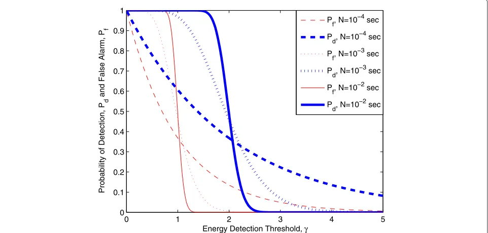
whereP(x,a)denotes the regularized lower gamma func-tion and is defined asP(x,a)= γ ((xa,a)) whereγ (x,a)is the lower incomplete gamma function and(a)is the Gamma function. In Figure 1, the probability of detection,Pd, and
the probability of false alarm,Pf, are plotted as a function
of the energy detection threshold,γ, for different values of channel detection duration. Note that the bandwidth isB = 10 kHz and the block duration isT = 0.1 s. We can see that when the detection threshold is low,Pdand
Pf tend to be 1, which means that the secondary user,
always assuming the existence of an active primary user, transmits with power P1(i) and rater1(i). On the other hand, when the detection threshold is high,PdandPf are
close to zero, which means that the secondary user, being unable to detect the activity of the primary users, always transmits with powerP2(i)and rater2(i), possibly caus-ing significant interference. The main purpose is to keep Pd as close to 1 as possible andPf as close to 0 as
possi-ble. Therefore, we have to keep the detection threshold in a reasonable interval. Note that the duration of detection is also important since increasing the number of channel samples used for sensing improves the quality of channel detection.
In the hypothesis testing problem in (3), another approach is to considerYkas Gaussian distributed, which
is accurate ifNBk is large [4]. In this case, the detection
and false alarm probabilities can be expressed in terms of GaussianQ-functions. We would like to note the rest of the analysis in the article does not depend on the specific expressions of the false alarm and detection probabilities. However, numerical results are obtained using (5) and (6).
State transition model
In this article, we assume that both the secondary receiver and transmitter have perfect channel side information, and hence perfectly know the realizations of the fading coefficients{hk(i)}. We further assume that the wideband
channel is divided into channels, each with bandwidth that is equal to the coherence bandwidthBc. Therefore,
we henceforth haveBk = Bc. With this assumption, we
can suppose that independent flat fading is experienced in each channel. In order to further simplify the setting, we consider a symmetric model in which fading coefficients are identically distributed in different channels. Moreover, we assume that the background noise and primary users’ signals are also identically distributed in different chan-nels and hence their variancesσn2andσs2p do not depend on k, and the prior probabilities of each channel being occupied by the primary users are the same and equal toρ. In channel sensing, the same energy threshold,γ, is applied in each channel. Finally, in this symmetric model, the transmission power and rate policies when the chan-nels are idle or busy are the same for each channel. Due to the consideration of a symmetric model, we in the subse-quent analysis drop the subscriptkin the expressions for the sake of brevity.
0 1 2 3 4 5
0 0.1 0.2 0.3 0.4 0.5 0.6 0.7 0.8 0.9 1
Energy Detection Threshold, γ
Probability of Detection, P
d
and False Alarm, P
f
Pf, N=10−4 sec
Pd, N=10−4 sec
P f, N=10
−3 sec
P d, N=10
−3 sec
P f, N=10
−2 sec
P d, N=10
−2 sec
First, note that we have the following four possible sce-narios considering the correct detections and errors in channel sensing:
Scenario 1:All channels are detected as busy, and chan-nel used for transmission is actually busy.
Scenario 2:All channels are detected as busy, and chan-nel used for transmission is actually idle.
Scenario 3:At least one channel is detected as idle, and channel used for transmission is actually busy.
Scenario 4:At least one channel is detected as idle, and channel used for transmission is actually idle.
In each scenario, we have one state, namely either ON or OFF, depending on whether or not the instanta-neous transmission rate exceeds the instantainstanta-neous chan-nel capacity. Considering the interferencesp(i)caused by
the primary users as additional Gaussian noise, we can express the instantaneous channel capacities in the above four scenarios as follows:
Scenario 1: C1(i)=Bclog2(1+SNR1(i)). Scenario 2: C2(i)=Bclog2(1+SNR2(i)). Scenario 3: C3(i)=Bclog2(1+SNR3(i)). Scenario 4: C4(i)=Bclog2(1+SNR4(i)).
Above, we have defined
SNR1(i)= P1(i)z(i)
Bc
σ2
n +σs2p
, SNR2(i)= P1(i)z(i)
Bcσn2
,
SNR3(i)=
P2(i)z(i)
Bc
σ2
n +σs2p
, SNR4(i)=
P2(i)z(i) Bcσn2
. (7)
Note thatz(i) = |h(i)|2 denotes the fading power. In scenarios 1 and 2, the secondary transmitter detects all channels as busy and transmits the information at rate
r1(i)=Bclog2(1+SNR1(i)). (8)
On the other hand, in scenarios 3 and 4, at least one channel is sensed as idle and the transmission rate is
r2(i)=Bclog2(1+SNR4(i)), (9)
since the transmitter, assuming the channel as idle, sets the power level toP2(i)and expects that no interference from the primary transmissions will be experienced at the secondary receiver (as seen by the absence ofσs2p in the denominator of SNR4).
In scenarios 1 and 2, transmission rate is less than or equal to the instantaneous channel capacity. Hence, reli-able transmission at rater1(i) is attained and channel is in the ON state. Similarly, the channel is in the ON state in scenario 4 in which the transmission rate isr2(i). On the other hand, in scenario 3, transmission rate exceeds the instantaneous channel capacity (i.e., r2(i) > C3(i)) due to miss-detection. In this case, reliable communica-tion cannot be established, and the channel is assumed to be in the OFF state. Note that the effective transmission rate in this state is zero, and therefore information needs to be retransmitted. We assume that this is accomplished through a simple ARQ mechanism.
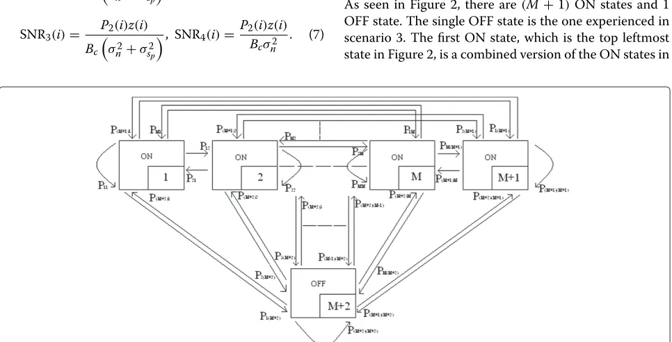
For this cognitive transmission model, we initially con-struct a state transition model. While the ensuing discus-sion describes this model, Figure 2 provides a depiction. As seen in Figure 2, there are(M+1)ON states and 1 OFF state. The single OFF state is the one experienced in scenario 3. The first ON state, which is the top leftmost state in Figure 2, is a combined version of the ON states in
scenarios 1 and 2 in both of which the transmission rate is r1(i)and the transmission power isP1(i). Note that all the channels are detected as busy in this first ON state. The remaining ON states labeled 2 through(M+1)can be seen as the expansion of the ON state in scenario 4 in which at least one channel is detected as idle and the channel cho-sen for transmission is actually idle. More specifically, the kth ON state fork =2, 3,. . .,(M+1)is the ON state in which(k−1)channels are detected as idle and the channel chosen for transmission is idle. Note that the transmission rate isr2(i)and the transmission power isP2(i)in all ON states labeled 2 through(M+1).
Next, we characterize the state transition probabilities. State transitions occur every T seconds. We can easily see that the probability of staying in the first ON state, in which all channels are detected as busy, is expressed as follows:
p11=αM (10)
whereα = ρPd+(1−ρ)Pf is the probability that
chan-nel is detected as busy, andPdandPf are the probabilities
of detection and false alarm, respectively, as defined in (6). Recall thatρdenotes the probability that a channel is busy (i.e., there are active primary users in the channel). It is important to note that the transition probability in (10) is obtained under the assumptions that the primary user activity is independent among the channels and also from one block to another. Indeed, under the assumption of independence over the blocks, the state transition prob-abilities do not depend on the originating stateaand hence we have
p11=p21= · · · =p(M+1)1=p(M+2)1=αMp1 (11)
where we have definedp1=pi1for alli=1, 2,. . .,M+2. Similarly, we can obtain fork=2, 3,. . .,M+1,
Now, we can easily observe that the transition probabil-ities for the OFF state are
p1(M+2)=p2(M+2)= · · · =p(M+1)(M+2)=p(M+2)(M+2) transition probability matrix can be expressed as
R=
Note thatRhas a rank of 1. Note also that in each frame duration ofT seconds,r1(k)(T−N)bits are transmitted and received in state 1, andr2(k)(T−N)bits are trans-mitted and received in states 2 through(M+1), while the transmitted number of bits is assumed to be zero in state
(M+2).
Interference power constraints
In this section, we consider interference power constraints to limit the transmission powers of the secondary users and provide protection to primary users. In particular, we assume that the transmission power of the secondary users is constrained in such a way that the average inter-ference power on the primary receiver is limited.
Note that interference to the primary users is caused in scenarios 1 and 3. In scenario 1, the channel is busy, and the secondary user, detecting the channel as busy,
p1k = p2k= · · · =p(M+1)k=p(M+2)k=P
(k−1)out ofM
channels are detected as idleandthe channel chosen for transmissionis actually idle
are detected as idle
× (1−ρ)(1−Pf) 1−α
probability that the channel chosen for transmission is actually idle given that it is detected as idle
transmits at power levelP1. Consequently, the instanta-neous interference power experienced by the primary user is P1zsp where zsp = |hsp(i)|2 is the magnitude-square
of the fading coefficient of the channel between the sec-ondary transmitter and the primary user. Note also that the probability of being in scenario 1 (i.e., the probabil-ity of detecting all channels busy and having the chosen transmission channel as actually busy) isα(M−1)ρPd, as
can easily be seen through an analysis similar to that in (13).
In scenario 3, the secondary user, detecting the chan-nel as idle, transmits at powerP2although the channel is actually is busy. In this case, the instantaneous interfer-ence power isP2zsp. Since we consider power adaption,
transmission power levelsP1andP2in general vary with zspand also withz, which is the power of the fading
coef-ficient between the secondary transmitter and secondary receiver in the chosen transmission channel. Hence, in both scenarios, the instantaneous interference power lev-els depend on bothzspandzwhose distributions depend
on the criterion with which the transmission channel is chosen and the number of available channels from which the selection is performed. For this reason, it is neces-sary in scenario 3 to separately consider the individual cases with different number of idle-detected channels. We haveMsuch cases. For instance, in thekth case fork = 1, 2,. . .,M, we havek channels detected as idle and the channel chosen out of thesek channels is actually busy. The probability of thekth case can easily be found to be
M!
(M−k)!k!α(M−k)(1−α)k−1ρ(1−Pd).
Following the above discussion, we can now express the average interference constraints as follows:
α(M−1)ρPd
probability of thekth case of scenario 3
× Ek
Note from above that Iavg is the constraint on the interference averaged over the distributions ofzandzsp
(through the expectations), and also averaged over the probabilities of different scenarios and cases. It is impor-tant to note that the termEk
P2zsp
, as discussed above, depends in general on the number of idle-detected chan-nels, k. This dependence is indicated through the sub-scriptk.
In a system with more strict requirements on the inter-ference, the following individual interference constraints can be imposed
interference averaged over fading is limited by the same constraint regardless of which scenario is being realized.
In the subsequent parts of the article, we assume that an average interference power constraint in the form given in (18) is imposed.
Effective capacity
In this section, we identify the maximum throughput that the cognitive radio channel with the aforementioned state-transition model can sustain under interference power constraints and statistical QoS limitations imposed in the form of buffer or delay violation probabilities.bWu and Negi [11] defined the effective capacity as the max-imum constant arrival rate that can be supported by a given channel service process while also satisfying a sta-tistical QoS requirement specified by the QoS exponent
θ. If we defineQas the stationary queue length, thenθ
is defined as the decay rate of the tail distribution of the queue lengthQ:
lim
q→∞
log Pr(Q≥q)
q = −θ. (20)
The effective capacity for a given QoS exponent θ is time, stationary, and ergodic stochastic service process. Note that(θ )is the asymptotic log-moment generating function ofS(t), and is given by
The service rate according to the model described in “State transition model” section isr(k)=r1(k)(T −N)if the cognitive system is in state 1 at timek. Similarly, the service rate isr(k)=r2(k)(T−N)in the states between 2 and(M+1). In the OFF state, instantaneous transmission rate exceeds the instantaneous channel capacity and reli-able communication cannot be achieved. Therefore, the service rate in this state is effectively zero.
In the next result, we provide the effective capac-ity for the cognitive radio channel and state transition model described in the previous section. This result is obtained by directly making use of the characterization in ([14],Chap. 7, Example 7.2.7), where effective bandwidth of Markov modulated processes is formulated.
Theorem 1.For the cognitive radio channel with the state transition model given in “State transition model” section, the normalized effective capacity (in bits/s/Hz) under the average interference power constraint (18) is given by
sition probabilities defined in (11), (15), and (17). Note also that the maximization is with respect to the power adaptation policies P1and P2.
Remark: In the effective capacity expression (23),
the expectation EP1zsp
in the constraint and Ee−(T−N)θr1are with respect to the joint distribution of
(z,zsp)of the channel selected for transmission when all
channels are detected busy. The expectationsEk
P2zsp
andEke−(T−N)θr2are with respect to the joint distri-bution of(z,zsp)of the channel selected for transmission
whenkchannels are detected as idle.
Proof of Theorem 1:In ([14],Chap. 7, Example 7.2.7), it is shown for Markov modulated processes that
(θ ) θ =
1
θ logesp(φ (θ )R) (24)
where sp(φ (θ )R) is the spectral radius (i.e., the maxi-mum of the absolute values of the eigenvalues) of the matrixφ (θ )R,Ris the transition matrix of the underlying Markov process, andφ (θ ) = diag(φ1(θ ),. . .,φ(M+2)(θ )) is a diagonal matrix whose components are the moment generating functions of the processes in given states. The rates supported by the cognitive radio channel with the state transition model described in the previous section can be seen as a Markov modulated process and hence the setup considered in [14] can immediately be applied to our setting. Since the processes in the states are time-varying transmission rates, we can easily find thatφ (θ )=
diagEe(T−N)θr1,E1e(T−N)θr2,. . .,EMe(T−N)θr2, 1.
Then, combining (26) with (24) and (21), normalizing the expression with TBc in order to have the effective
capacity in the units of bits/s/Hz, and considering the maximization over power adaptation policies, we reach to the effective capacity formula given in (23).
We would like to also note that the effective capacity expression in (23) is obtained for a given sensing duration N, detection thresholdγ, and QoS exponentθ. In the next section, we investigate the impact of these parameters on the effective capacity through numerical analysis. Before the numerical analysis, we first identify below the optimal power adaptation policies that the secondary users should employ.
Theorem 2.The optimal power adaptations for the secondary users under the constraint given in (18) are
P1= a parameter whose value can be found numerically by satisfying the constraint (18) with equality.
Proof.Since logarithm is a monotonic function, the optimal power adaptation policies can also be obtained from the following minimization problem:
min
It is clear that the objective function in (29) is strictly convex and the constraint function in (18) is linear with respect toP1andP2.cThen, forming the Lagrangian func-tion and setting the derivatives of the Lagrangian with respect toP1andP2equal to zero, we obtain
whereλis the Lagrange multiplier. Above,f(z,zsp)denotes
the joint distribution of(z,zsp)of the channel selected for
transmission when all channels are detected busy. Hence, in this case, the transmission channel is chosen amongM channels. Similarly,fk(z,zsp)denotes the joint distribution
whenkchannels are detected idle, and the transmission channel is selected out of thesekchannels. Definingβ1=
μ1ρPd
cα andβ2=
ρ(1−Pd)μ2
c(1−ρ)(1−Pf), and solving (30) and (31), we obtain the optimal power policies given in (27) and (28).
Now, using the optimal transmission policies given in (27) and (28), we can express the effective capacity as follows tations denote that the lower limits of the integrals are equal these values and not to zero. For instance,
Eβ1λ
Until now, we have not specified the criterion with which the transmission channel is selected from a set of available channels. In (32), we can easily observe that the effective capacity depends only on the channel power ratio
z
zsp, and is increasing with increasing
z tonically decreasing functions ofzz
sp. Therefore, the crite-rion for choosing the transmission band among multiple busy bands unless there is no idle band detected, or among multiple idle bands if there are idle bands detected should be based on this ratio of the channel gains. Clearly, the strategy that maximizes the effective capacity is to choose the channel (or equivalently the frequency band) with the highest ratio ofzz
sp. This is also intuitively appealing as we want to maximizezto improve the secondary transmis-sion and at the same time minimizezspto diminish the
interference caused to the primary users. Maximizing zz sp provides us the right balance in the channel selection.
We definex= maxi∈{1,2,...,M}zspzi,i where zzspi,i is the ratio
of the gains in theith channel. Assuming that these ratios are independent and identically distributed in different channels, we can express the pdf ofxas
fx(x)=Mf z
zsp andFzspz are the pdf and cumulative distribu-tion funcdistribu-tion (cdf ), respectively, of zz
sp, the gain ratio in
one channel. Now, the expectationEβ1λ
which arises under the assumption that all channels are detected busy and the transmission channel is selected among theseMchannels, can be evaluated with respect to the distribution in (33).
Similarly, we define xk = maxi∈{1,2,...,k}zspzi,i for k =
using the distribution in (34). Finally, after some calcula-tions, we can write the effective capacity in integral form as
In this section, we present numerical results for the effec-tive capacity as a function of the channel sensing reliability (i.e., detection and false alarm probabilities) and the aver-age interference constraints. Throughout the numerical results, we assume that QoS parameter isθ = 0.1, block duration isT =1 s, channel sensing duration isN=0.1 s, and the prior probability of each channel being busy is
ρ=0.1.
Before the numerical analysis, we first provide expres-sions for the probabilities of operating in each one of the four scenarios described in “State transition model” section. These probabilities are also important metrics in analyzing the performance. We have
In Figure 3, we plot these probabilities as a function of the detection probability Pd for two cases in which the
number of channels isM = 1 andM = 10, respectively. As expected, we observe thatPS1 andPS2 decrease with increasingM. We also see thatPS3 andPS4 are assuming small values whenPdis very close to 1. Note from Figure 1
that as Pd approaches 1, the false alarm probability Pf
increases as well.
Rayleigh fading
The analysis in the preceding sections apply for arbitrary joint distributions ofzandzspunder the mild assumption
that the they have finite means (i.e., fading has finite aver-age power). In this section, we consider a Rayleigh fading scenario in which the power gainszandzspare
exponen-tially distributed. We assume thatzandzsp are mutually
independent and each has unit-mean. Then, the pdf and cdf of zz
spcan be expressed as follows
f z
In Figure 4, we plot the effective capacity versus prob-ability of detection,Pd, for different number of channels
when the average interference power constraint
normal-ized by the noise power isI¯avg(dB) =10 log10
pis the noise variance at the primary user. We observe that with increasingPd, the effective
capac-ity is increasing due to the fact more reliable detection of the activity primary users leads to fewer miss-detections and hence the probability of scenario 3 or equivalently the probability of being in state (M+ 2), in which the transmission rate is effectively zero, diminishes. We also interestingly see that the highest effective capacity is attained when M = 1. Hence, secondary users seem to not benefit from the availability of multiple channels. This
P{secondary system is in scenario 1} =PS1 =α
probability that at least one channel is detected as idle
ρ(1−Pd)
1−α
probability that the channel chosen for transmission is actually busy
given that it is detected as idle
= (1−αM)ρ(1−Pd)
1−α , (36)
P{secondary system is in scenario 4} =PS4 =
(1−αM)(1−ρ)(1−Pf)
0 0.2 0.4 0.6 0.8 1 0
0.1 0.2 0.3 0.4 0.5 0.6 0.7 0.8 0.9 1
Proabability pf Scenarios
Probability of Detection, Pd P
S 1
, M = 1
P S
2 , M = 1
P S
3 , M = 1
PS 4
, M = 1
P S
1 , M = 10
P S
2 , M = 10
P S
3 , M = 10
PS 4
, M = 10
Figure 3Probability of different scenarios versus probability of detectionPdfor different number of channelsM.
is especially pronounced for high values ofPd. Although
several factors and parameters are in play in determin-ing the value of the effective capacity, one explanation for this observation is that the probabilities of scenar-ios 1 and 2, in which the secondary users transmit with powerP1, decrease with increasingM, while the proba-bilities of scenarios 3 and 4 increase as seen in (36). Note
that in scenario 3, no reliable communication is possible and transmission rate is effectively zero. In Figure 5, we display similar results whenI¯avg = −10 dB. Hence, sec-ondary users operate under more stringent interference constraints. In this case, we note thatM = 2 gives the highest throughput while the performance withM=1 is strictly suboptimal.
0 0.2 0.4 0.6 0.8 1
0.2 0.3 0.4 0.5 0.6 0.7 0.8
Probability of Detection, Pd
Effective Capacity (Bits/Sec/Hz)
M = 1 M = 5 M = 10 M = 20
0 0.2 0.4 0.6 0.8 1 0.2
0.3 0.4 0.5 0.6 0.7 0.8
Effective Capacity (Bits/Sec/Hz)
Probability of Detection, Pd M = 1
M = 2 M = 3 M = 5
Figure 5Effective capacity versus probability of detectionPdfor different number of channelsMwhen¯Iavg= −10dB.
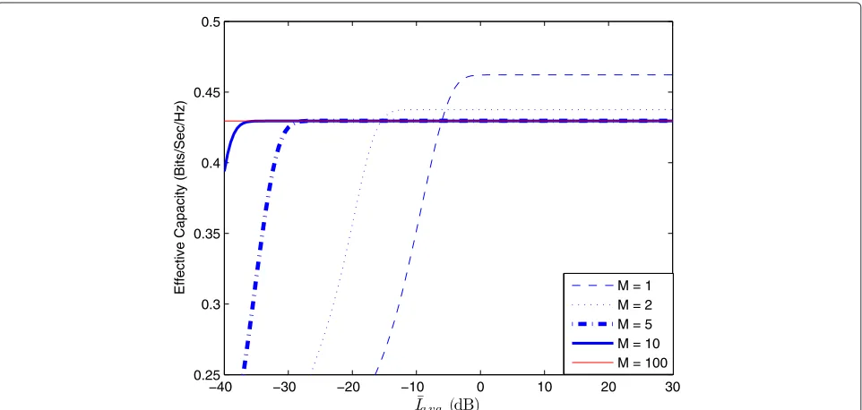
In Figure 6, we show the effective capacities as a func-tionI¯avg(dB) for different values ofMwhenPd =0.9 and
Pf =0.2. Confirming our previous observation, we notice
that as the interference constraint gets more strict and hence¯Iavgbecomes smaller, a higher value ofMis needed to maximize the effective capacity. For instance,M= 10 channels are needed when¯Iavg < −30 dB. On the other
hand, for approximatelyI¯avg>−6 dB, havingM=1 gives the highest throughput.
Above, we have remarked that increasing the number of available channels from which the transmission channel is selected provides no benefit or can even degrade the per-formance of secondary users under certain conditions. On the other hand, it is important to note that increasingM
−40 −30 −20 −10 0 10 20 30
0.25 0.3 0.35 0.4 0.45 0.5
Effective Capacity (Bits/Sec/Hz) M = 1
M = 2 M = 5 M = 10 M = 100
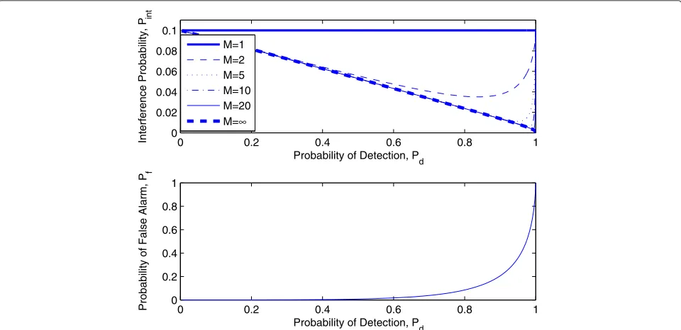
always brings a benefit to the primary users in the form of decreased probability of interference. In order to quan-tify this type of gain, we consider below the probability that the channel selected for transmission is actually busy and hence the primary user in this channel experiences interference
Pint=Pr
channel selected for transmission is actually busy
=Pr
channel selected for transmission is actually busy and
all channels are detected as busy
+Pr
channel selected for transmission is actually busy and
at least one channel is detected as idle
(38)
=PS1+PS3 (39)
=ρ1−α
M−P
d+Pdα(M−1)
1−α . (40)
Note thatPintdepends onPd and alsoPf throughα =
ρPd+(1−ρ)Pf. It can easily be seen that this
interfer-ence probabilityPint decreases with increasingMwhen Pd > Pf. AsMgoes to infinity, we have limM→∞Pint =
ρ1−Pd
1−α . Indeed, in this asymptotic regime, Pint becomes zero with perfect detection (i.e., withPd = 1). Note that
secondary users transmit (ifP1> 0) even when all chan-nels are detected as busy. AsM→ ∞, the probability of such an event vanishes. Also, havingPd = 1 enables the
secondary users to avoid scenario 3. Hence, interference is not caused to the primary users.
In Figure 7, we plotPintvs. the detection probability for
different values ofM. We also display how the false alarm probability evolves asPdvaries from 0 to 1. It can be easily
seen that whilePint = ρwhenM = 1, a smallerPint is
achieved for higher values of MunlessPd = 1. On the
other hand, as also discussed above, we immediately note thatPintmonotonically decreases to 0 asPdincreases to 1
whenMis unbounded (i.e.,M→ ∞).
Nakagami fading
Nakagami fading occurs when multipath scattering with relatively large delay-time spreads occurs. Therefore, Nak-agami distribution matches some empirical data better than many other distributions do. With this motiva-tion, we also consider Nakagami fading in our numerical results. The pdf of the Nakagami-mrandom variabley=
|h|is given byfy(y) = (2m)
m
2σ2 y
m
y2m−1e− my2
2σy2 wherem
is the number of degrees of freedom. If bothzspandzhave
the same number of degrees of freedom, we can express the pdf ofx= zz
sp as follows
fx(x)=
(2m)xm−1
(x+1)2m(m)2. (41)
Note also that Rayleigh fading is a special case of Nak-agami fading when m = 1. In our experiments, we
0 0.2 0.4 0.6 0.8 1
0 0.02 0.04 0.06 0.08 0.1
Probability of Detection, P d
Interference Probability, P
int
0 0.2 0.4 0.6 0.8 1
0 0.2 0.4 0.6 0.8 1
Probability of Detection, P d
Probability of False Alarm, P
f
M=1 M=2 M=5 M=10 M=20 M=∞
Figure 7Pintversus correct detection probabilityPdfor different number of channelsMin the upper figure.False alarm probabilityPf
consider the case in whichm = 3. Now, we can express the cdf ofxform=3 as
Fx(x)=1+
15
(x+1)4−
10
(x+1)3−
6
(x+1)4. (42)
In Figure 8, we plot effective capacity versus ¯Iavg (dB) for different values ofMwhenPd = 0.9 andPf = 0.2.
Here, we again observe results similar to those in Figure 6. We obtain higher throughput by sensing more than one channel in the presence of strict interference constraints on cognitive radios.
Conclusion
In this article, we have studied the performance of cogni-tive transmission under QoS constraints and interference limitations. We have considered a scenario in which sec-ondary users sense multiple channels and then select a single channel for transmission with rate and power that depend on both sensing decisions and fading. We have constructed a state transition model for this cognitive operation. We have meticulously identified possible sce-narios and states in which the secondary users operate. These states depend on sensing decisions, true nature of the channels’ being busy or idle, and transmission rates being smaller or greater than the instantaneous channel capacity values. We have formulated and imposed an aver-age interference constraint on the secondary users. Under such interference constraints and also statistical QoS limi-tations in the form of buffer constraints, we have obtained the maximum throughput through the effective capacity formulation. Therefore, we have effectively analyzed the
performance in a practically appealing setting in which both the primary and secondary users are provided with certain service guarantees. We have determined the opti-mal power adaptation strategies and the optiopti-mal chan-nel selection criterion in the sense of maximizing the effective capacity. We have had several interesting obser-vations through our numerical results. We have shown that improving the reliability of channel sensing expect-edly increases the throughput. We have noted that sens-ing multiple channels is beneficial only under relatively strict interference constraints. At the same time, we have remarked that sensing multiple channels can decrease the chances of a primary user being interfered.
Endnotes
aNote that under the block-fading assumption, there is no
memory in the state-transition model and hence the per-formance will depend on the steady-state probabilities of each state rather the transition probabilities.
bNote that interference constraints are imposed to
pro-vide a certain level of quality-of-service to the primary users, while buffer or delay constraints are used to statisti-cally guarantee a quality-of-service level to the transmis-sions of the secondary users. Hence, the formulation in the paper effectively considers service guarantees for both the primary and secondary users. On the other hand, QoS constraints throughout the paper refer to buffer/delay constraints to avoid confusion.
cStrict convexity follows from the strict concavity ofr 1and r2 in (8) and (9) with respect toP1andP2respectively,
−40 −30 −20 −10 0 10 20 30
0.3 0.32 0.34 0.36 0.38 0.4 0.42 0.44 0.46 0.48 0.5
Effective Capacity (Bits/Sec/Hz) M = 1
M = 2 M = 5 M = 10 M = 100
Figure 8Effective capacity versus¯Iavgfor different values ofMwhenPd=0.9andPf =0.2in the Nakagami-mfading channel with
strict convexity of the exponential function, and the fact that the nonnegative weighted sum of strictly convex functions is strictly convex ([15], Section 3.2.1).
Competing interests
The authors declare that they have no competing interests.
Acknowledgements
This study was supported by the National Science Foundation under Grants CNS-0834753 and CCF-0917265. The material in this article was presented in part at the IEEE International Conference on Communications (ICC), Cape Town, South Africa, May 2010.
Author details
1Institute of Communications Technology, Leibniz Universitat Hannover,¨ 30167 Hanover, Germany.2Department of Electrical Engineering and Computer Science, Syracuse University, Syracuse, NY 13244, USA.
Received: 26 July 2011 Accepted: 5 September 2012 Published: 24 September 2012
References
1. V Asghari, S Aissa, inIEEE International Conference on Communications. Rate and power adaptation for increasing spectrum efficiency in cognitive radio networks, (Dresden, Germany, 14–18 June 2009), pp. 1–5 2. L Musavian, S Aissa, Capacity and power allocation for spectrum-sharing
communications in fading channels. IEEE Trans. Wirel. Commun.8(1), 148–156 (2009)
3. A Ghasemi, E Sousa, Spectrum sensing in cognitive radio networks: the cooperation-processing tradeoff. Wirel. Commun. Mobile Comput.7(9), 1049–1060 (2007)
4. Y-C Liang, Y Zheng, ECY Peh, AT Hoang, Sensing-throughput tradeoff for cognitive radio networks. IEEE Trans. Wirel. Commun.7(4), 1326–1337 (2008)
5. Z Quan, S Cui, AH Sayed, HV Poor, inIEEE International Conference on Communications. Wideband spectrum sensing in cognitive radio networks, (Beijing, China, 19–23 May 2008), pp. 901–906
6. L Musavian, S Aissa, inIEEE International Conference on Communications. Adaptive modulation in spectrum-sharing systems with delay constraints, (Dresden, Germany, 14–18 June 2009), pp. 1822–1826
7. L Musavian, S Aissa, inIEEE Global Communication Conference.
Quality-of-service based power allocation in spectrum-sharing channels, (New Orleans, LA , USA, November 30–December 4, 2008), pp. 1–5 8. S Akin, MC Gursoy, Effective capacity analysis of cognitive radio channels
for quality of service provisioning. IEEE Trans. Wirel. Commun.9(11), 3354–3364 (2010)
9. S Akin, MC Gursoy, Performance analysis of cognitive radio systems under QoS constraints and channel uncertainty. IEEE Trans. Wirel. Commun. 10(9), 2883–2895 (2011)
10. HV Poor,An Introduction to Signal Detection and Estimation, 2nd edn. (Springer-Verlag, New York, 1994)
11. D Wu, R Negi, Effective capacity: a wireless link model for support of quality of service. IEEE Trans. Wirel. Commun.2(4), 630–643 (2003) 12. L Liu, J-F Chamberland, inIEEE International Symposium on Information
Theory. On the effective capacities of multiple-antenna Gaussian channels, (Toronto, Ontario, Canada, 6–11 July 2008), pp. 2583–2587 13. C-S Chang, T Zajic, inIEEE Infocom. Effective bandwidths of departure processes from queues with time varying capacities, (Boston, MA, USA, 2–6 April 1995), vol. 3, pp. 1001–1009
14. C-S Chang,Performance Guarantees in Communication Networks. (Springer, New York, 1995)
15. S Boyd, L Vandenberghe,Convex Optimization. (Cambridge University Press, Cambridge, UK, 2004)
doi:10.1186/1687-1499-2012-301
Cite this article as:Akin and Gursoy:Cognitive radio transmission under QoS constraints and interference limitations.EURASIP Journal on Wireless Communications and Networking20122012:301.
Submit your manuscript to a
journal and benefi t from:
7Convenient online submission 7 Rigorous peer review
7Immediate publication on acceptance 7 Open access: articles freely available online 7High visibility within the fi eld
7 Retaining the copyright to your article