On the approximation of time fractional telegraph equations using localized kernel based method

R E S E A R C H

Open Access

On the approximation of time-fractional

telegraph equations using localized

kernel-based method

Kamran

_{, Marjan Uddin}

_{and Amjad Ali}

*_{Correspondence:}

[email protected]

1_{Department of Mathematics,} Islamia College Peshawar, Khyber Pakhtoon Khwa, Pakistan Full list of author information is available at the end of the article

Abstract

In the present work, a hybrid transform-based localized meshless method is constructed for the solution of time-fractional telegraph equations. In the first step the Laplace transform is applied to the time-fractional telegraph equation, which reduces the problem to a finite set of elliptic equations which are solved with the help of local radial basis functions method in parallel. Finally, the solution is

represented as an integral along a smooth curve in the complex plane. The integral is then evaluated by quadrature rule. The advantage of this method is that it does not suffer from time instability that may occur in a time stepping procedure. A clear improvement is observed in terms of stability, accuracy and ill-conditioning.

Keywords: Laplace transform; Local kernel based method; Time-fractional telegraph equation

1 Introduction

Fractional calculus is the generalization of differentiation and integration to non-integer orders. Fractional calculus has gained special importance in the last two or three decades. Many phenomena in engineering and other sciences can be successfully modeled by frac-tional calculus [1–7]. The telegraph equations have many applications in physics and en-gineering. The applications arise, for example, in signal analysis [8], random walk theory [9], wave propagation [10].

The telegraph equations of fractional order have been investigated by many researchers. The solution of space–time-fractional telegraph equation in a bounded domain is ob-tained in terms of Mittage-Leffler functions by the method of generalized differential transform [11]. Das et al. [12] used a homotopy analysis method in approximating an an-alytical solution for the time-fractional telegraph equation and different particular cases have been derived. In [13] Jiang and Lin obtained a series solution for the time-fractional telegraph equation with Robin boundary value conditions using the reproducing kernel theorem. Saadatmandi and Mohabbati [14] have used the Tau method for the approxima-tion of fracapproxima-tional telegraph equaapproxima-tion. Liu et al. [15] derived the analytical solution of the nonhomogeneous time-fractional telegraph equation by considering three types of non-homogeneous boundary conditions using the method of separation of variables. In [16] the authors approximated the solution of fractional telegraph equation using radial basis

functions. More work on fractional telegraph equations can be found in [17–19], and the references therein.

In the present work, the Laplace transform is coupled with localized kernel-based method, and the resulting hybrid method is investigated for solving telegraph equations of fractional order. Following the work [20], the Bromwich integral associated with the inverse Laplace transform is approximated numerically with standard quadrature ofM

steps. By increasingM round off errors will occur which will make it difficult to find the true solution. The authors in [21] present a method that can safeguard against this. The combination of Laplace transform with some other methods have been successfully achieved earlier and is available in the literature, but only a small amount of work is avail-able. For example, the Laplace transform coupled with the boundary-particle method [22] and the Kansa method [23]. Similarly the authors of [24] studied the combination of Laplace transform with the RBF method on a unit sphere for solving the heat equation. The combination of Laplace transform with the finite element, the finite difference and the spectral methods can be found in Refs. [25–29]. We consider a time-fractional telegraph equation of fractional order 1₂<α≤1 of the form

CD2tαu(x,t) +λCDαtu(x,t) =μLu(x,t) +f(x,t), x∈⊂Rd,d≥1, (1.1) subject to initial and boundary conditions

u(x, 0) =ϕ1(x), ut(x, 0) =ϕ2(x), x∈, (1.2)

and

Bu(x,t) =g1(t), x∈∂, (1.3)

respectively, whereLis a linear spatial differential operator andBis a boundary differen-tial operator andCDαt is the Caputo fractional partial derivative of orderα.

2 Preliminaries

In this section, we give some important definitions about fractional calculus.

Definition 2.1 Let the Laplace transform ofu(t) be defined by

Lu(t)=U(z) =

_∞

0

e–ztu(t)dt. (2.1)

Definition 2.2 The Riemann–Liouville derivative of fractional orderαof a functionu(t) is defined as (see [30])

RLDαtu(t) = 1

(p–α)

dp dtp

t

0

(t–s)p–α–1u(s)ds, (2.2)

Definition 2.3 The Caputo fractional partial derivative of orderα of a functionu(t) is the Caputo fractional derivative is given by

LCDαtu(t)

In this section, we propose a meshless method based on Laplace transform for time-fractional telegraph equation. In the proposed method we eliminate the time variable by a Laplace transform and for the time independent PDE, the localized meshless numerical scheme will be constructed.

Applying the Laplace transform to Eqs. (1.1)–(1.3), we get

z2αU(x,z) –z2α–1ϕ1(x) –z2α–2ϕ2(x) +λ

Thus we have the following system of linear differential equations:

z2αI+λzαI–μL U(x,z)=G(x,z), x∈, (3.3)

BU(x,z)=G1(z), x∈∂, (3.4)

where

G(x,z) =z2α–1ϕ1(x) +z2α–2ϕ2(x) +λzα–1ϕ1(x) +F(x,z).

In the next section the kernel-based method in local setting is employed to approximate the governing differential operatorsLand the boundary differential operator Band to solve the time independent problem (3.3)–(3.4) in Laplace space.

3.1 Spatial discretization via local kernel based method

whereαi_{= [α}i

1,αi2, . . . ,αin] is the expansion coefficients vector, andr=xi– xhis the dis-tance between centers xiand xh,ψ(r),r≥0 is a radial kernel andi⊂is a local domain for each center xi, containingnneighboring centers around xi. Thus we haveNsmall size linear systems of ordern×ngiven by

Ui= iαi, i= 1, 2, . . . ,N, (3.6)

the entries of i arebi_lh=ψ(xl– xh), xl, xh ∈i, the matrix i is known as the in-terpolation matrix, we need to solve each small size n×n system for the unknowns αi_{= [α}i

1,αi2, . . . ,αin]. Next theLU(x), is approximated by LU(xi) =

xh∈i

αi_hLψx_i– xh

, (3.7)

Equation (3.7) can be written as a product of two vectors, given by

LU(xi) = vi·αi, (3.8)

whereαi_{of ordern×1 is a vector of unknown coefficients, and v}i_{is a vector of order 1×n} with entries given by

vi=Lψxi– xh

, xh∈i, (3.9)

using Eq. (3.6), we eliminate the unknown coefficients,

αi= i–1Ui, (3.10)

and by inserting the values ofαifrom (3.10) in (3.8) we get

LU(xi) = vi i–1Ui= wiUi, (3.11)

where

wi= vi i–1. (3.12)

Hence for each center, the localized approximation of the linear differential operator L using radial basis functions is given by

LU≡DU. (3.13)

3.2 Choosing optimal shape parameter

In the literature we can find a variety of kernel functions. In this work the multiquadrics,

ψ(r) =1 + (εr)2_{are selected. These kernels contain a scale factorεand accuracy of the}

solution relies upon this scale factor. For an optimal value of this scale factor εa large amount of work is available in the literature [31–35] and the references therein. In this paper we utilize the uncertainty principle [36] (e.g., a better accuracy can be achieved comparatively at larger condition numbers of these type of kernel based system matrices) for a decent estimation of the scale factorε.

Algorithm

• The condition number is kept approximately in the range1012_{<κ< 10}16_{for our} problem system matrices.

• Decompose the interpolation matrix asQ, S, V =svd( i_{)using a singular value}

decomposition. The interpolation matrix i_{is of ordern×nfor each local}

subdomaini, andSis diagonal matrix containingnsingular values of i, and

κ= i₍ i₎–1_{=max(S)/min(S)denotes the condition number of the matrix} i_.

• Search forεuntilκsatisfy the condition1012<κ< 1016, using the algorithm

κ= 1

When the above condition is satisfied a good value ofεis obtained, the inverse is computed using( i)–1= (QSVT₎–1_{= VS}–1_QT_{[37]. Thus we can computew}i_in

(3.12).

After discretization of the operatorsLandBby a localized meshless method the system (3.3)–(3.4) is solved for each point along the contour of integrationz. Then the solution

u(x,t) of problem (1.1)–(1.3) can be obtained by the inverse Laplace transform

The approximation of (3.16) can be obtained by the trapezoidal rule with uniform step

4 Error analysis of the method

The accuracy of the approximate solution defined by (3.17) is based on the choice of con-tour. In the literature various such contours are available, for example parabolic [20] and hyperbolic [27]. We used the hyperbolic contour in our computation due to [27]:

z(η) =ω+λ1 –sin(δ–ιη), forη∈R, () (4.1)

withλ> 0,ω≥0, 0 <δ<β–1₂π, and1₂π<β<π. In fact, whenImη=γ, (4.1) reduces to the left branch of the hyperbola

To discuss the stability of system (3.3)–(3.4), in discrete form this system may be repre-sented as

AU= b, (5.1)

whereAisN×Nsparse differentiation matrix which can be obtained by localized kernel-based method discussed in Sect.3. the stability constant corresponding to system (5.1) is given by

C=sup

U=0

U

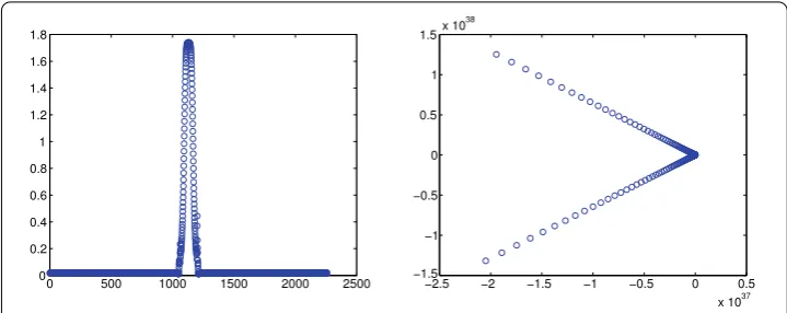
Figure 1First plot show the stability constantCof our differentiation matrixAfor various points along the hyperbolic path. The second plot shows the hyperbolic path, corresponding to Problem 1

whereCis finite using any type of discrete norms · onRN_{. The above equation can be} expressed as

A–1≤ U

AU≤C. (5.3)

Again in terms of the pseudoinverseA†ofA, we have

A†=sup

v=0

A†v

v . (5.4)

Now we write

A†≥ sup

v=AU=0

A†_AU AU =supU=0

U

AU=C. (5.5)

Hence Eqs. (5.3) and (5.5) ensure the boundedness of the stability constantC. For a nu-merical approximation of the system (5.1) the calculation of the pseudoinverse may be computationally expansive, but it ensures numerical stability. In the case of square sys-tems, the MATLAB’s function condest estimatesA–1∞, thus we have

C=condest(A ₎

A∞ . (5.6)

This works well for our sparse matrixAwith a small amount of computations. The bounds of stability constantCof our system (3.3)–(3.4) corresponding to Problem 1 are shown in Fig. 1. Choosing M= 90,N= 50 andn= 7 at timet= 1, we can see that 0.0088≤

C≤1.7401, which shows the stability constant is bounded by numbers that are not very large, and this implies the numerical stability of localized kernel-based numerical scheme.

6 Numerical results

The accuracy of the solution depends on the shape parameterε. A number of criteria are available in the literature for choosing optimal values of the shape parameters. We use the uncertainty principle due to [36] to select the optimal shape parameter. The accu-racy of the proposed method is measured by the maximum absolute error (L∞) defined by

L∞=u(x,t) –uk(x,t)_∞= max

1≤j≤N

u(x,t) –uk(x,t).

Hereuandukdenotes the exact and approximate solutions, respectively. The error norms are calculated at fixed value oftin time interval [t0,T], wheret0andT are given in each numerical experiment.

6.1 Problem 1

Here we apply our proposed numerical method to the one dimensional time-fractional telegraph equation [13],

Different quadrature points are used along the hyperbolic contour. These points are generated by MATLAB statementη= –M:k:Mfor hyperbolic contour. The param-eters used areθ= 0.1,δ= 0.1541,r= 0.1387,ω= 2,t0= 0.5 andT= 5. The other optimal parameters are given in (4.1). TheL∞error and error estimate (E) using fractional orders

α= 0.8, 0.96 are shown in Table1. Various numbers of pointsNin the global domain

Table 1 The maximum absolute error in our method and in [13] corresponding to Problem 1

M L_∞error E ε κ CPU time (s)

α= 0.8,N= 30,n= 5 5 4.7135 7.2328 0.8 1.0508e+012 0.136899

7 0.2062 5.9685 0.8 1.0508e+012 0.140582

10 0.0025 4.4187 0.8 1.0508e+012 0.139019

25 0.0019 0.9164 0.8 1.0508e+012 0.165614

30 3.9156e–004 0.5373 0.8 1.0508e+012 0.188401 50 1.7714e–004 0.0625 0.8 1.0508e+012 0.352443 70 1.6868e–004 0.0072 0.8 1.0508e+012 0.789112 90 1.6856e–004 8.1825e–004 0.8 1.0508e+012 1.967992

[13] 5.60e–005

α= 0.96,N= 50,n= 7 5 6.0719 7.2328 3 1.0041e+012 0.136641

7 0.2656 5.9685 3 1.0041e+012 0.142100

10 0.0034 4.4187 3 1.0041e+012 0.146196

25 0.0023 0.9164 3 1.0041e+012 0.207502

30 6.2477e–004 0.5373 3 1.0041e+012 0.249881

50 1.1877e–004 0.0625 3 1.0041e+012 0.648773

70 1.1406e–004 0.0072 3 1.0041e+012 1.786508

90 1.1400e–004 8.1825e–004 3 1.0041e+012 5.400089

[13] 2.10e–004

we can approximate the telegraph equation very accurately in time without any time in-stability issue. The local nature of the method makes it more attractive for such a type of problems.

6.2 Problem 2

Next we consider the one dimensional time-fractional telegraph equation withα=2₃,

CD2tαu(x,t) +CDαtu(x,t) =D2xu(x,t) +f(x,t), 0 <x< 1, 0 <t≤1,

over the domain [0, 1] at timet= 1. Various quadrature points along the hyperbolic path

Table 2 The maximum absolute error, shape parameter, condition number and computational time corresponding to Problem 2 att= 1

α=2₃,N= 45,n= 5 M L∞error E ε κ CPU time(s)

10 1.8374 4.4187 1.2 1.1509e+012 0.145084

20 0.3122 1.5582 1.2 1.1509e+012 0.159080

35 0.0373 0.3144 1.2 1.1509e+012 0.255237

50 0.0075 0.0625 1.2 1.1509e+012 0.539619

70 4.1395e–004 0.0072 1.2 1.1509e+012 1.361986

90 6.0201e–005 8.1825e–004 1.2 1.1509e+012 4.342044

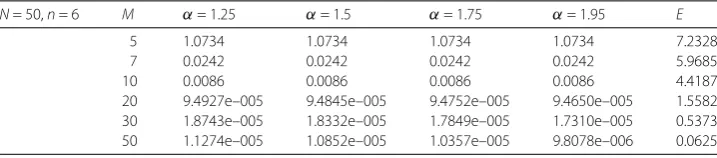
Table 3 The maximum absolute error for differentM,N,nandαcorresponding to Problem 3 att= 1

N= 50,n= 6 M α= 1.25 α= 1.5 α= 1.75 α= 1.95 E

5 1.0734 1.0734 1.0734 1.0734 7.2328

7 0.0242 0.0242 0.0242 0.0242 5.9685

10 0.0086 0.0086 0.0086 0.0086 4.4187

20 9.4927e–005 9.4845e–005 9.4752e–005 9.4650e–005 1.5582 30 1.8743e–005 1.8332e–005 1.7849e–005 1.7310e–005 0.5373 50 1.1274e–005 1.0852e–005 1.0357e–005 9.8078e–006 0.0625

andnin the local domainiare used. The shape parameter is optimized using the un-certainty principle [36]. The condition number κ, the shape parameterεand the CPU time(s) are given in Table2. A similar performance is observed to the one we observed in Problem 1.

6.3 Problem 3

As a third example we consider the one dimensional time-fractional telegraph equation withα∈(1, 2] [16]

CDαtu(x,t) +CDtα–1u(x,t) +u(x,t) =πD2xu(x,t) +f(x,t), 0 <x< 1, 0 <t≤1,

where

f(x,t) = 6sin(x)2

t3–α

(4 –α)+

t4–α

(5 –α)+

t3

6

– 2πt3cos(2x),

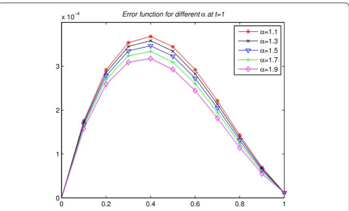
subject to the initial conditionu(x, 0) =ut(x, 0) = 0, 0 <x< 1, and the boundary conditions are chosen according to the exact solutionu(x,t) =t3_(sin(x))2_{. Here we tested our method}

Figure 2Error function forN= 11,n= 4,M= 70 and differentαatt= 1 corresponding to Problem 3

6.4 Problem 4

In the last example we consider the one dimensional time-fractional telegraph equation withα∈(1, 2] [38]

CDαtu(x,t) +CDtα–1u(x,t) +u(x,t) =D2xu(x,t) +f(x,t), 0 <x< 1, 0 <t≤1,

where

f(x,t) =

t2–α

(3 –α)+t

x2–x– 2t

subject to the initial condition

u(x, 0) =ut(x, 0) =x2–x, 0 <x< 1,

and the boundary conditions are

u(0,t) =u(1,t) = 0.

Exact solution of the problem isu(x,t) = (x2_{–x)t. The problem is solved over the domain}

[0, 1] at timet= 1. The same hyperbolic contourand the same optimal parameters are used in this problem. The absolute errors and error estimate for the contourare shown in Table4using fractional orderα= 1.95. The result given in Table4shows that the pro-posed method is accurate and efficient as compared to [38]. So the proposed method is an excellent alternative for solving the fractional order telegraph equations.

7 Conclusion

Table 4 The maximum absolute error of the proposed method for different values ofMandN= 11,

any time instability, which is commonly encountered in time stepping mesh-free meth-ods. These time stepping methods require a very small time step for greater accuracy on the expense of large computations. We tested our procedure for 1D telegraph equa-tions with time-fractional orders. The accuracy and performance of the methods is ex-cellent for solving time-fractional telegraph equations. The proposed hybrid mesh-free method is an excellent alternative for solving time-fractional partial differential equa-tions.

Acknowledgements

The authors would like to thank the reviewers for their valuable comments.

Funding

This work is self-supported by the authors in respect of funding and technically supported by Islamia College Peshawar and University of Engineering and Technology, Khyber Pakhtun Khwa, Peshawar, Pakistan.

Competing interests

The authors declare that they have no conflict of interests.

Authors’ contributions

All the authors contributed in theoretical and computational results and all authors read and approved the final manuscript.

Author details

1_{Department of Mathematics, Islamia College Peshawar, Khyber Pakhtoon Khwa, Pakistan.}2_{Department of Basic Sciences}

and Islamiat, University of Engineering and Technology Peshawar, Khyber Pakhtoon Khwa, Pakistan.

Publisher’s Note

Springer Nature remains neutral with regard to jurisdictional claims in published maps and institutional affiliations.

References

1. Baleanu, D., Muslih, S.I., Ta¸s, K.: Fractional Hamiltonian analysis of higher order derivatives systems. J. Math. Phys. 47(10), 103503 (2006)

2. Aguilar, J.F., Córdova-Fraga, T., Tórres-Jiménez, J., Escobar-Jiménez, R.F., Olivares-Peregrino, V.H., Guerrero-Ramírez, G.V.: Nonlocal transport processes and the fractional Cattaneo–Vernotte equation. Math. Probl. Eng.2016, Article ID 7845874 (2016).https://doi.org/10.1155/2016/7845874

3. Gómez-Aguilar, J.F., Escobar-Jiménez, R.F., López-López, M.G., Alvarado-Martínez, V.M.: Atangana–Baleanu fractional derivative applied to electromagnetic waves in dielectric media. J. Electromagn. Waves Appl.30(15), 1937–1952 (2016)

4. Coronel-Escamilla, A., Gómez-Aguilar, J.F., Alvarado-Méndez, E., Guerrero-Ramírez, G.V., Escobar-Jiménez, R.F.: Fractional dynamics of charged particles in magnetic fields. Int. J. Mod. Phys. C27(08), 1650084 (2016)

5. Coronel-Escamilla, A., Gómez-Aguilar, J.F., Baleanu, D., Córdova-Fraga, T., Escobar-Jiménez, R.F., Olivares-Peregrino, V.H., Qurashi, M.M.Al.: Bateman–Feshbach tikochinsky and Caldirola–Kanai oscillators with new fractional differentiation. Entropy19(2), 55 (2017)

6. Gomez-Aguilar, J.F., Yepez-Martinez, H., Torres-Jiménez, J., Córdova-Fraga, T., Escobar-Jimenez, R.F., Olivares-Peregrino, V.H.: Homotopy perturbation transform method for nonlinear differential equations involving to fractional operator with exponential kernel. Adv. Differ. Equ.2017(1), 68 (2017)

7. Morales-Delgado, V.F., Taneco-Hernández, M.A., Gómez-Aguilar, J.F.: On the solutions of fractional order of evolution equations. Eur. Phys. J. Plus132(1), 47 (2017)

8. Jordan, P.M., Puri, A.: Digital signal propagation in dispersive media. J. Appl. Phys.85, 1273–1282 (1999)

9. Banasiak, J., Mika, J.R.: Singular perturbed telegraph equations with applications in the random walk theory. J. Appl. Math. Stoch. Anal.11, 9–28 (1998)

10. Weston, V.H., He, S.: Wave splitting of the telegraph equation inr3_{and its application to inverse scattering. Inverse}

Probl.9, 789–812 (1993)

11. Garg, M., Manohar, P., Kalla, S.L.: Generalized differential transform method to space–time fractional telegraph equation. Int. J. Differ. Equ. Appl.2011, Article ID 548982 (2011).https://doi.org/10.1155/2011/548982

12. Das, S., Vishal, K., Gupta, P.K., Yildirim, A.: An approximate analytical solution of time-fractional telegraph equation. Appl. Math. Comput.217(18), 7405–7411 (2011)

13. Jiang, W., Lin, Y.: Representation of exact solution for the time-fractional telegraph equation in the reproducing kernel space. Commun. Nonlinear Sci. Numer. Simul.16, 3639–3645 (2011)

14. Saadatmandi, A., Mohabbati, M.: Numerical solution of fractional telegraph equation via the Tau method. Math. Rep. 17(67)(2), 155–166 (2015)

15. Chen, J., Liu, F., Anh, V.: Analytical solution for the time-fractional telegraph equation. J. Math. Anal. Appl.338, 1364–1377 (2008)

16. Hosseini, V.R., Chen, W., Avazzadeh, Z.: Numerical solution of fractional telegraph equation by using radial basis functions. Eng. Anal. Bound. Elem.38, 31–39 (2014)

17. Beghin, L., Orsingher, E.: The telegraph process stopped at stable distributed times and its connection with the fractional telegraph equation. Fract. Calc. Appl. Anal.6(2), 187–204 (2003)

18. Orsingher, E., Zhao, X.: The space-fractional telegraph equation and the related fractional telegraph process. Chin. Ann. Math.1, 45–56 (2003)

19. Orsingher, E., Beghin, L.: Time-fractional telegraph equations and telegraph processes with Brownian time. Probab. Theory Relat. Fields128(1), 141–160 (2004)

20. Weideman, J.A.C., Trefethen, L.N.: Parabolic and hyperbolic contours for computing the Bromwich integral. Math. Comput.76(259), 1341–1356 (2007)

21. Schäle, A., Fernandez, M.L., Lubich, C.: Fast and oblivious convolution quadrature. SIAM J. Sci. Comput.28(2), 421–438 (2006)

22. Fu, Z.J., Chen, W., Yang, H.T.: Boundary particle method for Laplace transformed time fractional diffusion equations. J. Comput. Phys.235, 52–66 (2013)

23. Moridis, G.J., Kansa, E.J.: The Laplace transform multiquadric method: a highly accurate scheme for the numerical solution of partial differential equations. J. Appl. Sci. Comput.1, 375–475 (1994)

24. Gia, Q.T.L., Mclean, W.: Solving the heat equation on the unit sphere via Laplace transforms and radial basis functions. Adv. Comput. Math.40(2), 353–375 (2014)

25. Sheen, D., Shaon, I.H., Thomee, V.: A parallel method for time discretization of parabolic equations based on Laplace transformation and quadrature. IMA J. Numer. Anal.23(2), 269–299 (2003)

26. McLean, W., Thomee, V.: Time discretization of an evolution equation via Laplace transforms. IMA J. Numer. Anal.24, 439–463 (2004)

27. McLean, W., Thomee, V.: Numerical solution via Laplace transforms of a fractional order evolution equation. J. Integral Equ. Appl.22(1), 57–94 (2010)

28. Fernandez, M.L., Palencia, C.: On the numerical inversion of the Laplace transform of certain holomorphic mappings. Appl. Numer. Math.51(2), 289–303 (2004)

29. Jacobs, B.A.: High-order compact finite difference and Laplace transform method for the solution of time fractional heat equations with Dirichlet and Neumann boundary conditions. Numer. Methods Partial Differ. Equ.32, 1184–1199 (2016)

30. Oldham, K.B., Spanier, J.: The Fractional Calculus Theory and Applications of Differentiation and Integration to Arbitrary Order, vol. 111. Academic Press, New York, London (1974)

31. Uddin, M.: On the selection of a good value of shape parameter in solving time dependent partial differential equations using RBF approximation method. Appl. Math. Model.38(1), 135–144 (2014)

32. Carlson, R.E., Foley, T.A.: The parameterr2_{in multiquadric interpolation. Comput. Math. Appl.21(9), 29–42 (2014)}

33. Foley, T.A.: Near optimal parameter selection for multiquadric interpolation. Manuscript, Computer Science and Engineering Department, Arizona State University, Tempe (1994)

35. Fasshauer, G.E., Zhang, J.G.: On choosing optimal shape paramters for RBF approximation. Numer. Algorithms 45(1–4), 345–368 (2007)

36. Schaback, R.: Error estimates and condition numbers for radial basis function interpolation. Adv. Comput. Math.3, 251–264 (1995)

37. Trefethen, L.N., Bau, D.: Numerical Linear Algebra. Other Titles in Applied Mathematics, vol. 50. SIAM, Philadelphia (1997)