Dynamical analysis of a ratio dependent predator–prey model with Holling III type functional response and nonlinear harvesting in a random environment

(1)

R E S E A R C H

Open Access

Dynamical analysis of a ratio-dependent

predator–prey model with Holling III type

functional response and nonlinear harvesting

in a random environment

Guijie Lan

1

_{, Yingjie Fu}

1

_{, Chunjin Wei}

1

_{and Shuwen Zhang}

1*

*_{Correspondence:} [email protected] 1_{School of Science, Jimei University,} Xiamen, China

Abstract

The objective of this paper is to study the dynamics of the stochastic ratio-dependent predator–prey model with Holling III type functional response and nonlinear

harvesting. For the autonomous system, sufficient conditions for globally positive solution and stochastic permanence are established. Then, applying comparison theorem for stochastic differential equation, sufficient conditions for extinction and persistence in the mean are obtained. In addition, we prove that there exists a unique stationary distribution and it has ergodicity under certain parametric restrictions. For the periodic system, we obtain conditions for the existence of a nontrivial positive periodic solution. Finally, numerical simulations are carried out to substantiate the analytical results.

Keywords: Predator–prey system; Harvesting; Stochastic permanence; Stationary

distribution and ergodicity; Positive periodic solution

1 Introduction

Renewable resources (such as ﬁsheries and forestry resources) are considered to be inex-haustible at all times, but excessive exploitation will actually exhaust them. The optimal management of renewable resources, which has a direct relationship to sustainable de-velopment, has been studied extensively by many authors (see [1, 2] and the references cited therein). Xiao [1] pointed out that the aim is to determine how much we can har-vest without dangerously altering the harhar-vested population. According to Clark in [2], the management of renewable resources has been based on the maximum sustainable yield, with the property that any larger harvest rate will lead to the depletion of the population. Thus, it is important to investigate the reasonable exploitation of renewable resources and their eﬀective utilization to obtain the maximum revenue.

In recent years, the harvesting eﬀects on the dynamics of predator–prey systems have attracted lots of attention and considerable work has been done (see [3–8] and the ref-erences cited therein). In their papers, an adequate amount of thorough investigation is carried out to study the existence of periodic solutions for biological models with harvest-ing terms. For example, Hou [4] discussed a ratio-dependent predator–prey system with

(2)

multiple harvesting terms. By means of using coincidence degree theory, they established the existence of at least four positive periodic solutions for the system. Wei [5] discussed a three-species periodic predator–prey system with Holling III type functional response and harvesting terms. By means of using coincidence degree theory, they established the existence of at least eight positive periodic solutions for the system. In addition, Gupta et al. [9] presented three types of harvesting functions (constant harvesting, proportional harvesting, nonlinear harvesting), and showed that nonlinear harvesting is more realis-tic than constant harvesting and proportional harvesting. Motivated by [1–11], in this paper, we propose the following ratio-dependent predator–prey system with Holling III type functional response and nonlinear harvesting terms, which therefore is described as:

_dx(t)

dt =x(t)(r1–a1x(t) –

b1x(t)y(t)

x2_(t)+my2_(t)–

f1

1+w1x(t)), dy(t)

dt =y(t)(r2– b2y(t)

k2+x(t)–

f2

1+w2y(t)),

(1.1)

wherex(t) andy(t) represent the population densities at timet, respectively. All param-eters involved in the model are positive. The paramparam-eters have the following biological meanings:r1andr2 are intrinsic growth rates of the prey and predator species, respec-tively. a1 denotes the density-dependent coeﬃcient of the prey. The associated ratio-dependent form of the Holling type III functional response is b1x2(t)y(t)

x2_(t)+my2_(t), whereb1stands for the conversion rates,mfor half capturing saturation [11]. The meaning ofb2is similar tob1,k2measures the extent to which environment provides protection for predatory.

f1x

1+w1x(t),

f2y

1+w2y(t) are both nonlinear harvesting terms wherefi(i= 1, 2) is the catchability

coeﬃcient,wi(i= 1, 2) is the suitable positive constant [9].

(3)

arose nearby. Hence, the constant catchability coeﬃcientfi(i= 1, 2) is replaced by a ran-dom variablefi+σidBi(t) (i= 1, 2), whereB1(t),B2(t) are mutually independent Brownian motions,σ₁2,σ₂2represent the intensities of the white noise. Then, corresponding to the deterministic model (1.1), the stochastic system takes the following form:

dx(t) =x(t)(r1–a1x(t) –_x2b_(t)+my1x(t)y(t)2_(t)–

f1

1+w1x(t))dt–

σ1x(t)

1+w1x(t)dB1(t),

dy(t) =y(t)(r2–_kb₂2_+x(t)y(t) –_1+wf2₂_y(t))dt–_1+wσ2y(t)₂_y(t)dB2(t).

(1.2)

In the article, we focus on the eﬀects of environmental noise and harvests on the dynam-ics of the system (1.2). On the other hand, periodic behavior arises naturally in many real world problems such as in biological, environmental, and economic systems. To better un-derstand the dynamic behavior of the population, numerous authors consider the eﬀects of periodic variation and stochasticity (see [23, 29] and the references cited therein). In this paper, we will consider the periodic behavior in the following stochastic model:

dx(t) =x(t)(r1(t) –a1(t)x(t) – b1(t)x(t)y(t)

x2_(t)+m(t)y2_(t)–

f1(t)

1+w1(t)x(t))dt–

σ1(t)x(t)

1+w1(t)x(t)dB1(t),

dy(t) =y(t)(r2(t) –_kb₂2_(t)+x(t)(t)y(t) –_1+wf₂2(t)_(t)y(t))dt–_1+wσ2(t)y(t)₂_(t)y(t)dB2(t),

(1.3)

wherer1(t),a1(t),b1(t),m(t),f1(t),w1(t),σ1(t),r2(t),b2(t),k2(t),f2(t),w2(t),σ2(t) are all positiveT-periodic continuous functions. We will obtain the existence of the periodic Markov process of system (1.3) by the method of Khasminskii [30].

The rest of the paper is organized as follows. In Sect. 2, we give the existence and unique-ness of global positive solution and the solution is stochastically ultimately bounded. Moreover, we obtain that stochastic system (1.2) is stochastically permanent in Sect. 3. In Sect. 4, suﬃcient conditions for extinction, stochastic persistence in the mean of the population are established. In Sect. 5, we show the existence of a unique stationary distri-bution and ergodicity. The existence of a positive periodic solution for non-autonomous periodic solution is also obtained in Sect. 6. Finally, the conclusions are given and our main results are illustrated through numerical simulations.

2 Existence and uniqueness of globally positive solution

Throughout this paper, unless otherwise speciﬁed, we let (,F,{Ft}t≥0,P) be a complete probability space with a ﬁltration {Ft}t≥0satisfying the usual conditions (i.e., it is right continuous andF0contains all P-null sets). For convenience we introduce the notations

Rn₊=X(t) = (x1,x2, . . . ,xn)∈Rn|xi> 0 for all 1≤i≤n

, X(t)= n

i=1

x2 i.

Iff(t) is integrable, we deﬁnef(t)T=_T1 T

0 f(t)dt,T > 0. And iff(t) is bounded, we deﬁnefu₌_sup

t∈[0,+∞)f(t),fl=inft∈[0,+∞)f(t).

(4)

and then, by constructing some suitable Lyapunov function, we prove that this solution is global. Explanation for ‘explosion time’ used in the following lemma can be found in [31].

Lemma 2.1 For(x(0),y(0))∈R2

+,there is a unique positive local solution(x(t),y(t))of

sys-tem(1.2)for t∈[0,τe)a.s.,whereτeis the explosion time.

Proof Letu(t) =lnx(t) andv(t) =lny(t), by use of Itô’s formula, we get that

⎧ ⎨ ⎩

du(t) = [r1–a1eu– b1e

u+v

e2u_+me2v –

f1

1+w1eu–

σ₁2

2(1+w1eu)2]dt–

σ1

1+w1eudB1(t),

dv(t) = [r2– b2e

v

k2+eu–

f2

1+w2ev–

σ₂2

2(1+w2ev)2]dt–

σ2

1+w2evdB2(t),

(2.1)

subjected to the initial conditionu(0) =logx(0),v(0) =logy(0). The functions involved in a drift part of the stochastic differential system above satisfy the linear growth condition and are locally Lipschitz. Hence there exists a unique local solution (u(t),v(t)) fort∈[0,τe), whereτe is any finite positive real number. Clearly,x(t) =eu(t),y(t) =ev(t) is the unique positive local solution of stochastic differential system (1.2) starting from an interior point

of the ﬁrst quadrant.

Now we are in a position to show that this unique solution is not only a local solution but a global solution. To prove this, we need to show thatτe=∞a.s.

Theorem 2.1 For any given initial value (x(0),y(0))∈R2

+, there is a unique solution (x(t),y(t))to system (1.2),and the solution will remain in R2

+with probability1,that is, (x(t),y(t))∈R2

+for all t≥0almost surely.

Proof Letk0 > 0 be suﬃciently large for (x(0),y(0)) lying within the interval [_k1₀,k0]× [_k1

0,k0]. For each integerk≥k0, deﬁne the stopping time

τk=inf

t∈[0,τe) :x(t) /∈

1

k,k

;y(t) /∈

1

k,k

.

Throughout this paper we setinf∅=∞(as usual,∅denotes the empty set). Clearly,τkis increasing ask→ ∞. Setτ∞=limk→∞τk, henceτ∞≤τea.s. If we can show thatτ∞=∞ a.s., thenτe=∞a.s. and (x(t),y(t))∈R2+a.s. for allt≥0. In other words, to complete the proof, all we need to show is thatτ∞=∞a.s. For if this statement is false, then there is a pair of constantsT> 0 andε∈(0, 1) such that

P{τ∞≤T}>ε, (2.2)

hence, there is an integerk1≥k0such thatP{τk≤T} ≥εfor allk≥k1. Deﬁne aC2-functionV:R2₊→R+as follows:

(5)

whereV1=x–lnx,V2=y–lny,V3= (k2+x)y. By Itô’s formula we have

Moreover, we also have

LV3= (k2+x)y

In fact, one can see that

(6)

Integrating both sides of (2.3) from 0 toτk∧Tyields

Vx(τk∧T),y(τk∧T)

≤Vx(0),y(0)+ τk∧T

0

C2ds+M1+M2, (2.5)

where

M1= τk∧T

0

1 –1

x+y

σ1x 1 +w1x

dB1, M2=

τk∧T

0

1 –1

y+k2+x

σ2y 1 +w2y

dB2.

Taking expectations of both sides of (2.5) yields

EVx(τk∧T),y(τk∧T)

≤Vx(0),y(0)+C2(τk∧T). (2.6)

Setk={τk≤T}fork≥k1and by (2.2)P(k)≥ε. Note that for everyω∈k such thatx(τk,ω) ory(τk,ω) equals eitherkor 1_k, and henceV is no less than eitherk–lnkor

1

k+lnk. Consequently,

Vx(τk,ω),y(τk,ω)

≥(k–lnk)∧

1

k+lnk

.

It then follows from (2.6) that

Vx(0),y(0)+C2T≥E

1k(ω)V

X(τk,ω)

≥ε(k–lnk)∧

1

k+lnk

,

where 1_kis the indicator function ofk. Lettingk→ ∞leads to the contradiction

∞>Vx(0),y(0)+C2T=∞.

So we must haveτ∞=∞. The conclusion is conﬁrmed.

Theorem 2.1 shows that the solutions to system (1.2) will remain inR2

+. The property makes us continue to discuss how the solution varies inR2

+in more detail. We ﬁrst present the deﬁnition of stochastic ultimate boundedness which is one of the important topics in population dynamics.

Deﬁnition 2.1([32]) The solutionX(t) = (x(t),y(t)) of Eq. (1.2) is said to be stochastically ultimately bounded if for anyε∈(0, 1) there is a positive constantδ=δ(ε) such that, for any initial valueX(0)∈R2₊, the solutionX(t) to (1.2) has the property that

lim sup

t→∞

PX(t) >δ<ε.

Theorem 2.2 The solutions of system(1.2)are stochastically ultimately bounded for any

(7)

Proof From Theorem 2.1, the solutionX(t) will remain inR2

+for allt≥0 with probabil-ity 1. Let us deﬁne aC2_-function_V_:_R2

+→R+as follows:

V=x2+y2+ (k2+x)y2.

Applying Itô’s formula, we obtain

LV = 2x2

r1–a1x–

b1xy

x2₊_my2 –

f1 1 +w1x

+ σ

2 1x2 (1 +w1x)2

+ 2y2

r2–

b2y

k2+x – f2

1 +w2y

+ σ 2 2y2 (1 +w2y)2

+ (k2+x)2y2

r2–

b2y

k2+x – f2

1 +w2y

+ (k2+x)

σ₂2y2 (1 +w2y)2

+xy2

r1–a1x–

b1xy

x2₊_my2–

f1 1 +w1x

≤–2a1x3+ 2r1x2+σ12+ 2r2y2+σ22– 2b2y3–a1x2y2

+ 2r2(k2+x)y2+ (k2+x)σ22+r1xy2.

Deﬁne the function

W=etV.

Applying Itô’s formula, we have

LW =et(V+LV)

≤etx2+y2+ (k2+x)y2– 2a1x3+ 2r1x2+σ12+ 2r2y2+σ22

– 2b2y3–a1x2y2+ 2r2(k2+x)y2+ (k2+x)σ22+r1xy2

.

Similar to the proof of Eq. (2.3), there exists a constantC3such thatLW≤C3et. Therefore

dW≤C3etdt–et

2x+y2 σ1x

1 +w1x

dB1– 2et(1 +k2+x)y

σ2y 1 +w2y

dB2. (2.7)

Integrating and taking expectations of both sides of (2.7) from 0 tot, yields

Eetx2+y2+ (k2+x)y2

≤W(0) +C3

et– 1,

i.e.,

Ex2+y2+ (k2+x)y2

≤W(0)e–t+C3

1 –e–t.

It is straightforward to see that

E2|X|<EX2=Ex2+y2≤Ex2+y2+ (k2+x)y2

≤W(0)e–t+C3

1 –e–t,

i.e.,E(|X|) has an upper bound. To proceed, applying the Chebyshev inequality yields the

(8)

3 Stochastic permanence

Generally speaking, the non-explosion property, the existence, and the uniqueness of the solution are not enough, but the property of permanence is more desirable since it means the long time survival in population dynamics. Now, the deﬁnition of stochastic perma-nence will be given below [32].

(9)

(10)

Note that (x+y)θ_≤₂θ₍_x2₊_y2₎2θ _{= 2}θ|_X|θ_{, where}_X_{= (}_x_,_y₎∈_R2

+. Consequently,

lim sup

t→∞ E

1

|X|θ

≤2θC4

k .

The proof is completed.

Theorem 3.2 If system(1.2)satisﬁesmin{r1,r2}–max{b1+f2,f1}–

(θ+1)max{σ₁2,σ2 2}

2 > 0,where 0 <θ< 2,then Eq. (1.2)is stochastically permanent.

The proof is the application of the well-known Chebyshev inequality, Theorems 2.2 and 3.1. Here it is omitted.

4 Stochastic persistence in the mean and extinction

Let us continue to discuss the long time behavior of stochastic model (1.2). From the point of view of the optimal management of renewable resources, how much can we harvest without dangerously altering the harvested population? On the other hand, how much will larger harvest rate lead to the depletion of the population? In this section, we will show that stochastic system (1.2) may preserve some important dynamics of the origi-nal deterministic system without harvesting terms when the intensities of noises and the catchability coefficient are small. On the contrary, if the catchability coefficient is suffi-ciently large, the populations will become extinct with probability one. Now, we present the definition of persistence in the mean and extinction.

Deﬁnition 4.1([33]) System (1.2) is said to be persistent in the mean if

lim inf

t→∞ 1

t

0

x(s)ds> 0 a.s., lim inf

t→∞ 1

t

0

y(s)ds> 0 a.s.

Deﬁnition 4.2([33]) The populationx(t) is said to go to extinction if

lim

t→∞x(t) = 0 a.s.

Lemma 4.1 Assume that(x(t),y(t))is the positive solution of Eq. (1.2)with the initial value

(x(0),y(0)).If r1>₂√b1_m+f1+ σ₁2

2 ,then we have

lim

t→∞

lnx(t)

t ≥0 a.s.

Proof Applying Itô’s formula to Eq. (1.2), we can see

1

x(t)= 1

x(0)e –r1t+0t

b1xy x2+my2+

f1 1+w₁x

σ₁2

2(1+w1x)2ds+

t

0

σ1 1+w₁xdB1

+a1e –r1t+0t

b1xy x2+my2+

f1 1+w₁x

σ₁2

2(1+w1x)2ds+

t

0

σ1 1+w₁xdB1

×

t

0

er1s–

s

0

b₁xy x2+my2+

f₁

1+w1x

σ₁2

2(1+w₁x)2dτ–

s

0

σ1 1+w1xdB1

ds

(11)

By computation, we get

Similar to the proof of [33] (Theorem 3.1), we obtain

lim

t→∞

lnx(t)

t ≥0 a.s.

Next, we consider the following stochastic model:

Proof By the ﬁrst equation of (4.1), we represent the solution. And there exists a constant

(12)

≤ 1

Similar to the proof of [33], we obtain

lim sup

t→∞

ln(t)

t ≤0 a.s.

On the other hand,

1

Similar to the proof of [33], we obtain

lim

Theorem 4.1 Suppose f1<r1–₂√b1_m – σ₁2

2,f2<r2– σ₂2

2 are satisﬁed,and x(t),y(t)is the

positive solution to Eq. (1.2)with initial value x(0) > 0,y(0) > 0,then the system is persistent in the mean.

Proof By comparison theorem for stochastic diﬀerential equation, Lemma 4.1 and

Lemma 4.2, one can see that

(13)

Applying Itô’s formula to Eq. (1.2), we have

Integrating both sides from 0 tot, one can see that

ln x(t)

Theorem 4.2 Suppose x(t),y(t)is the positive solution to Eq. (1.2)with initial value x(0) >

Proof (i) Deﬁne Lyapunov functionslnx, by Itô’s formula, one can see that

lnx(t) –lnx(0) =

Integrating both sides from 0 totand dividing byt, one can see that

(14)

Hence, for arbitrary smallε> 0, there existt0and a setεsuch thatP(ε)≥1 –εand

one can see that

y

According to Theorem 4.1, it is easy to see that

lim

(ii) Applying Itô’s formula to Eq. (4.2), one can get that

dlny=

5 A sufﬁcient condition for stationary distribution

In this section, we prove the existence of stationary distribution of the prey and predator populations. The stationary solution means that it is a stationary Markov process which shows that the prey and predator can be persistent and will not die out in the population. For this purpose, we ﬁnd the stationary distribution for solutions of system (1.2), which in turn imply the stability in stochastic sense. Before proving the main theorem related to the stationary distribution, we state a useful lemma from [30] which will be useful to prove the theorem.

(15)

equa-tions:

dX(t) =b(X)dt+ k

s=1

gs(X)dBs(t). (5.1)

Deﬁnition 5.1([15, 34]) Denote byPγ the corresponding probability distribution of an

initial distributionγ, which describes the initial state of model (5.1) att= 0. Suppose that the distribution ofX(t) with initial distributionγconverges in some sense to a distribution

π=πγ (a prioriπmay depend on the initial distributionγ), i.e.,

lim

t→∞Pγ

X(t)∈F=π(F)

for all measurableF, then we say that model (5.1) has a stationary distributionπ(·).

The diﬀusion matrix is deﬁned by [30],

A(x) =aij(x), aij(x) = k

s=1

gi_s(x)g_sj(x).

We assume that there exists a bounded domainU⊂Elwith regular boundary, bearing the following properties:

(P1) In the domainU and some neighborhood thereof, the smallest eigenvalue of the diﬀusion matrixA(x)is bounded away from zero.

(P2) Ifx∈El\U, the mean timeτ at which a path emerging fromxreaches the setUis

ﬁnite, andsup_x_∈_KExτ<∞for every compact subsetK⊂El.

Lemma 5.1 If assumptions(P1)and(P2)above hold,then the Markov process X(t)has a

stationary distributionμ(·).Let f(·)be a function integrable with respect to the measure μ(·).Then

Px

lim

T→∞ 1

T

0

fX(t)dt=

El

f(x)μ(dx)

= 1 for all x∈El.

To validate (P1), it is suﬃcient to prove thatLis uniformly elliptical inU, whereLV =

b(X)VX+trA(X)V₂ XX, i.e., there is a positive numberGsuch that

l

i,j=1

aij(x)ξiξj≥G|ξ|2 for allx∈U,ξ∈Rl.

To validate (P2), it is enough to show that there exist some neighborhoodUand a non-negativeC2_-function_V _{such that, for any}_x_∈_E

l\U,LV(x) is negative.

Theorem 5.1 Assume f1<r1–σ12–2√b1m,f2<r2–σ 2

2.Then,for any initial value(x0,y0)∈

R2

+,there exists a unique stationary distributionμ(·)for system(1.2),and it has ergodic

(16)

Proof We have known that for any initial value (x(0),y(0))∈R2

+, there is a unique solution (x(t),y(t))∈R2

By Itô’s formula one may calculate the operatorLV

LV = –1

In fact, according to the proof of Eq. (2.3), there existsC5> 0 such that

–a1x

To conﬁrm the condition (P2) of Lemma 5.1, we consider the bounded open subset

U1,2={(x,y)∈R2+|1<x<11,2<y<

For convenience, we divideUC

1,2into four domains

(17)

Case 1.On domainU1, we get

LV ≤–r1–f1–σ 2 1–2√b1m

x –

r2–f2–σ22

y –

a1x2 2 –

b2y2 2 +C5

≤–r1–f1–σ 2 1–2√b1m

1

+C5

≤–1.

Case 2.On domainU2, one can see that

LV ≤–r1–f1–

σ2 1–

b1

2√m

x –

r2–f2–σ22

y –

a1x2 2 –

b2y2 2 +C5

≤–r2–f2–σ 2 2

2

+C5

≤–1.

Case 3.On domainU3it yields

LV ≤–r1–f1–

σ₁2– b1

2√m

x –

r2–f2–σ22

y –

a1x2 2 –

b2y2 2 +C5

≤–a1 –2 1 2 +C5

≤–1.

Case 4.On domainU4, one can get that

LV ≤–r1–f1–

σ2 1–2√b1m

x –

r2–f2–σ22

y –

a1x2 2 –

b2y2 2 +C5

≤–b2 –2 2 2 +C5

≤–1.

Consequently,

LV(x,y)≤–1 for∀(x,y)∈UC1,2,

that is, the condition (P2) holds.

On the other hand, we takeU1to be a neighborhood ofU1,2withU1⊆R2+. There is

M= min

(x,y)∈U1

σ₁2x2 (1 +w1x)2

, σ 2 2y2 (1 +w2y)2

> 0

such that

2

i,j=1

aij(x,y)ξiξj=

σ₁2x2 (1 +w1x)2

ξ₁2+ σ 2 2y2 (1 +w2y)2

(18)

for all (x,y)∈U1,ξ = (ξ1,ξ2)∈R2

+, which means that the condition (P1) of Lemma 5.1 is satisﬁed. Therefore, according to Lemma 5.1, we know that the system is ergodic and pos-itive recurrent. And system (1.2) has a unique stationary distributionμ(·). The conclusion

is conﬁrmed.

6 The existence of periodic solution of non-autonomous system

In what follows, we ﬁrst recall a basic deﬁnition and introduce a lemma which gives criteria for the existence of a periodic Markov process (see Khasminskii [30]).

Deﬁnition 6.1([30]) A stochastic processξ(t) =ξ(t,ω) (–∞<t< +∞) is said to beT

-periodic if for every ﬁnite sequence of numberst1,t2, . . . ,tn, the joint distribution of ran-dom variablesξ(t1+h),ξ(t2+h), . . . ,ξ(tn+h) is independent ofh, whereh=kT(k= 1, 2, . . .).

Consider the integral equation

X(t) =X(t0) + t

t0

bs,X(s)ds+ k

r=1 t

t0

σr

s,X(s)dξr(s), (6.1)

whereb(s,x),σi(s,x) (i= 1, 2, . . . ,k) (s∈[t0,T],x∈Rl) are continuous functions of (s,x) and for some constantB, the following conditions hold:

b(s,x) –b(s,y)+ k

r=1

σr(s,x),σr(s,y)≤B|x–y|,

b(s,x)+ k

r=1

σr(s,x)≤B

1 +|x|.

(6.2)

Lemma 6.1([30]) Suppose that the coeﬃcients of(6.1)are T -periodic in t and satisfy

con-ditions(6.2)in every cylinder I×U,and assume further there exists a function V(t,x)∈C2

which is T -periodic in t and satisﬁes: (Q1) inf|x|>RV(t,x)→ ∞,

(Q2) LV(t,x)≤–1outside some compact set.

Then system (6.1) has at least aT-periodic Markov process.

Theorem 6.1 Ifr1(t) –f1(t) –σ12(t) –₂√b1_m(t)(t) T> 0,r2(t) –f2(t) –σ22(t)T> 0,then system (1.3)has one positive T -periodic solution.

Proof By the same way as in Theorem 2.1 one can see that, for any initial (x,y)∈R2 +, system (1.3) has a unique global positive solution (x,y)∈R2₊, we only need to verify the conditions (Q1), (Q2) of Lemma 6.1.

Deﬁne aC2,1_-function_V₍_x_,_y_,_t_{) :}_R2

+×R+→R+as follows:

V(x,y,t) =e θ1(t)

x1 +e

θ2(t)

x2

(19)

where

According to the proof of Eq. (2.3), there existsC6> 0 such that

(20)

Consider the bounded open subset

D1,2=

(x,y)1<x< 1

1

,2<y< 1

2

,

where 0 <i< 1 is a suﬃciently small number. In the setDC1,2=R

2

+\D1,2, let us choose

suﬃciently smallisuch that

1≤min

_eθ1(t)_r

1(t) –f1(t) – ₂b√1_m(t)(t) –σ12(t)T

C6+ 1

l ,

a1 2(C6+ 1)

l ,

2≤min

eθ2(t)_r

2(t) –f2(t) –σ22(t)T

C6+ 1

l ,

b2 2(C6+ 1)

l .

For convenience, we divideDC

1,2into four domains:

D1=

(x,y)∈R2₊|0 <x≤1

, D2=

(x,y)∈R2₊|0 <y≤2

,

D3=

(x,y)∈R2₊x≥ 1 1

, D4=

(x,y)∈R2₊1≤x≤ 1

1 ,y≥ 1

2

.

Clearly,DC

1,2=D1∪D2∪D3∪D4. Similar to the proof of Theorem 5.1, we obtain that

LV(x,y,t)≤–1 for any (x,y,t)∈DC

1,2×R+. By Lemma 6.1, periodic system (1.3) has a

periodic solution. The result is conﬁrmed.

7 Numerical simulations and conclusion

In this paper, we have considered the basic features of a ratio-dependent predator–prey model with Holling III type functional response and nonlinear harvesting in presence of white noise terms to understand the dynamics in presence of environmental driv-ing forces. Although we are considerdriv-ing a predator–prey model, the survival of preda-tor species in absence of the prey population is justified as we have assumed that the predators have alternative food source and their growth follows the logistic growth law. For the autonomous system, we have established the existence of positive global solu-tion of the stochastic model. Moreover, we show that the positive solusolu-tions are stochas-tically bounded. The sufficient conditions for stochastic permanence, stochastic persis-tence in the mean, and extinction are established. Then, by constructing some suitable Lyapunov function, the existence of stationary distribution for both populations is es-tablished under certain parametric restrictions. These parametric restrictions reflect the idea that large amplitude environmental noise can destabilize the system, and in that sit-uation one cannot find any stationary distribution. The result shows that stationary dis-tribution does not rely on the existence and the stability of the positive equilibrium in the deterministic system. There is a periodic phenomenon in a non-autonomous peri-odic system: when r1(t) –f1(t) –σ2

1(t) – b1(t)

2√m(t)T > 0, r2(t) –f2(t) –σ 2

(21)

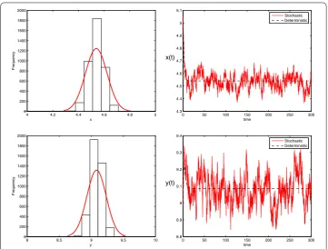
Figure 1The left is density function diagrams of system (1.2); the right is the solutions of stochastic system (1.2) and its corresponding deterministic system (1.1) with initial value (x(0),y(0)) = (4.5, 9). The parameters are taken as Eq. (7.1) andσ1= 0.02,σ2= 0.02,f1= 0.06,f2= 0.06

For numerical simulations of the stochastic model (1.2), we choose the parameters as

r1= 0.5, a1= 0.1, b1= 0.1, m= 4, w1= 1

6, r2= 0.5,

b2= 0.5, k2= 5, and w2= 1 6.

(7.1)

Then we take account of the white noise and the catchability coeﬃcient which have eﬀects on the prey and predator populations. The numerical scheme obtained through Milstein’s method applied to the stochastic model under consideration is given by

⎧ ⎨ ⎩

xi+1=xi+xi[r1–a1xi–_xb21xiyi

i+my2i

– f1

1+w1xi]t–

σ1xi

1+w1xi

√ tξi+

σ₁2xi

2(1+w1xi)2(ξ

2 i – 1)t,

yi+1=yi+yi[r2–_kb₂2_+xyi_i–_1+wf2₂_y_i]t–_1+wσ2y₂i_y_i

√ tηi+

σ₂2yi

2(1+w2yi)2(η

2 i – 1)t,

whereξiandηi(i= 1, 2, . . . ,n) are independent Gaussian random variables which follow

N(0, 1) [35].

We start our numerical simulation with environmental forcing intensities σ1= 0.02,

(22)

Figure 2The left is density function diagrams of system (1.2); the right is the solutions of stochastic system (1.2) and its corresponding deterministic system (1.1) with initial value (x(0),y(0)) = (4.5, 9). The parameters are taken as Eq. (7.1) andσ1=σ2= 0.2,f1=f2= 0.06

Figure 3Numerical simulation for system (1.1) and (1.2) with initial value (x(0),y(0)) = (4.5, 9). The parameters are taken as Eq. (7.1) andσ1=σ2= 0.2,f1=f2= 0.6 shows that both prey and predator populations go to extinction

predator population is also provided in Fig. 1. From stationary distribution of two popula-tions, it is clear that they are distributed normally around the mean values 4.55 and 9.08, respectively.

(23)

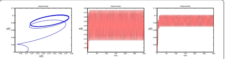
Figure 4The left is a sample phase portrait of system (1.3); middle and right are the solutions of stochastic system (1.3) with initial value (x(0),y(0)) = (4.5, 9). The parameters are taken as Eq. (7.2) andσ1=σ2= 0

Figure 5The left is a sample phase portrait of system (1.3); middle and right are the solutions of stochastic system (1.3) with initial value (x(0),y(0)) = (4.5, 9). The parameters are taken as Eq. (7.2) and

σ1=σ2= 0.001 + 0.0001 sin(t)

more compared to the earlier case. This ﬂuctuation is also reﬂected at the stationary dis-tribution as the prey population is distributed within (2, 7) and the predator population within the range (6, 12) (see Fig. 2). From Figs. 1 and 2, we conclude that, as the noise intensity decreases, the variability of the stochastic model decreases and approaches the deterministic model dynamics.

If we chooseσ1= 0.2,σ2= 0.2,f1= 0.6, andf2= 0.6, then the second condition of The-orem 4.2 will be satisﬁed. As a result, the prey as well as the predator population go to extinction (see Fig. 3). It tell us that overharvesting will lead to the depletion of the popu-lation.

For numerical simulations of the stochastic model (1.3), we choose the parameters as follows:

r1= 0.5 + 0.002sin(t), a1= 0.1 + 0.002sin(t), b1= 0.1 + 0.002sin(t),

m= 4 + 0.002sin(t), w1= 1

6+ 0.002sin(t), r2= 0.5 + 0.002sin(t),

b2= 0.5 + 0.002sin(t), k2= 5 + 0.002sin(t), w2= 1

6+ 0.002sin(t),

f1= 0.06 + 0.002sin(t), f2= 0.06 + 0.002sin(t),

(7.2)

and the initial values are taken as (4.5, 9). Then we use diﬀerent values ofσ1,σ2in order to understand the role of the noise strength on the resulting dynamics for system (1.3). We start our numerical simulation with two diﬀerent noise intensities:

(24)

persistent in the mean and has a periodic solution. Results of one simulation run are re-ported in Figs. 4 and 5. One can see that, for any positive initial value, the solution of the deterministic system will enter the periodic orbit after a period of time, and the solution of the stochastic system is ﬂuctuating in a small neighborhood of the periodic orbit when the noise intensity is small.

Results of simulations run reveal that the forcing intensity of ﬂuctuating environment and catchability play a crucial role behind the survival of prey and predator species.

Acknowledgements

This research was supported by the Fujian provincial Natural science of China (No. 2016J01667, 2016J05012). Competing interests

The authors declare that they have no competing interests. Authors’ contributions

SZ and CW suggested the model, helped in result interpretation, manuscript evaluation, and supervised the

development of work. GL and YF helped to evaluate, revise, and edit the manuscript. All authors read and approved the ﬁnal manuscript.

Publisher’s Note

Springer Nature remains neutral with regard to jurisdictional claims in published maps and institutional aﬃliations.

Received: 18 January 2018 Accepted: 28 April 2018

References

1. Xiao, D., Jennings, L.S.: Bifurcations of a ratio-dependent predator–prey system with constant rate harvesting. SIAM J. Appl. Math.65, 737–753 (2005)

2. Clark, C.W.: The optimal management of renewable resources. Nat. Resour. Model.43, 31–52 (1990)

3. Zhao, K., Ye, Y.: Four positive periodic solutions to a periodic Lotka–Volterra predatory–prey system with harvesting terms. Nonlinear Anal., Real World Appl.11, 2448–2455 (2010)

4. Zhang, Z., Hou, Z.: Existence of four positive periodic solutions for a ratio-dependent predator–prey system with multiple exploited (or harvesting) terms. Nonlinear Anal., Real World Appl.11, 1560–1571 (2010)

5. Wei, F.: Existence of multiple positive periodic solutions to a periodic predator–prey system with harvesting terms and Holling III type functional response. Commun. Nonlinear Sci. Numer. Simul.16, 2130–2138 (2011)

6. Li, Z., Zhao, K., Li, Y.: Multiple positive periodic solutions for a non-autonomous stage-structured predatory–prey system with harvesting terms. Commun. Nonlinear Sci. Numer. Simul.15, 2140–2148 (2010)

7. Hu, D., Zhang, Z.: Four positive periodic solutions to a Lotka–Volterra cooperative system with harvesting terms. Nonlinear Anal., Real World Appl.11, 1115–1121 (2010)

8. Zhang, N., Chen, F., Su, Q., et al.: Dynamic behaviors of a harvesting Leslie–Gower predator–prey model. Discrete Dyn. Nat. Soc.2011, 309–323 (2011)

9. Gupta, R., Chandra, P., Banerjee, M.: Dynamical complexity of prey–predator model with nonlinear predator harvesting. Discrete Contin. Dyn. Syst., Ser. A20, 423–443 (2015)

10. Ling, L., Wang, W.: Dynamics of a Ivlev-type predator–prey system with constant rate harvesting. Chaos Solitons Fractals41, 2139–2153 (2009)

11. Wang, L., Li, W.: Periodic solutions and permanence for a delayed nonautonomous ratio-dependent predator–prey model with Holling type functional response. J. Comput. Appl. Math.162, 341–357 (2004)

12. May, R., Macdonald, N.: Stability and Complexity in Model Ecosystems. IEEE Trans. Syst. Man Cybern., vol. 8 (2007) 13. Britton, T.: Stochastic epidemic models: a survey. Math. Biosci.225, 24–35 (2010)

14. Wang, W., Cai, Y., Li, J., et al.: Periodic behavior in a FIV model with seasonality as well as environment ﬂuctuations. J. Franklin Inst.354, 7410–7428 (2017)

15. Cai, Y., Kang, Y., Wang, W.: A stochastic SIRS epidemic model with nonlinear incidence rate. Appl. Math. Comput.305, 221–240 (2017)

16. Fu, J., Han, Q., Lin, Y., et al.: Asymptotic behavior of a multigroup SIS epidemic model with stochastic perturbation. Adv. Diﬀer. Equ.2015, Article ID 84 (2015)

17. Cao, B., Shan, M., Zhang, Q., et al.: A stochastic SIS epidemic model with vaccination. Physica A486, 127–143 (2017) 18. Guo, W., Cai, Y., Zhang, Q., et al.: Stochastic persistence and stationary distribution in an SIS epidemic model with

media coverage. Physica A492, 2220–2236 (2018)

19. Cai, Y., Jiao, J., Gui, Z., et al.: Environmental variability in a stochastic epidemic model. Appl. Math. Comput.329, 210–226 (2018)

20. Li, W., Wang, K.: Optimal harvesting policy for stochastic logistic population model. Appl. Math. Comput.218, 157–162 (2011)

21. Liu, M., Bai, C.: Optimal harvesting policy of a stochastic food chain population model. Appl. Math. Comput.245, 265–270 (2014)

(25)

23. Zuo, W., Jiang, D.: Stationary distribution and periodic solution for stochastic predator–prey systems with nonlinear predator harvesting. Commun. Nonlinear Sci. Numer. Simul.36, 65–80 (2016)

24. Mandal, P.: Noise-induced extinction for a ratio-dependent predator–prey model with strong Allee eﬀect in prey. Physica A496, 40–52 (2018)

25. Mandal, P., Banerjee, M.: Stochastic persistence and stationary distribution in a Holling–Tanner type prey–predator model. Physica A391, 1216–1233 (2012)

26. Liu, Q., Jiang, D., Hayat, T., et al.: Stationary distribution and extinction of a stochastic predator–prey model with additional food and nonlinear perturbation. Appl. Math. Comput.320, 226–239 (2018)

27. Zhang, Q., Wen, X., Jiang, D., et al.: The stability of a predator–prey system with linear mass-action functional response perturbed by white noise. Adv. Diﬀer. Equ.2016, Article ID 54 (2016)

28. Liu, Q., Jiang, D.: Stationary distribution and extinction of a stochastic predator–prey model with distributed delay. Appl. Math. Lett.78, 79–87 (2018)

29. Jiang, D., Zhang, Q., Hayat, T., et al.: Periodic solution for a stochastic non-autonomous competitive Lotka-Volterra model in a polluted environment. Physica A471, 276–287 (2017)

30. Khasminskii, R.: Stochastic Stability of Differential Equations. Monographs and Textbooks on Mechanics of Solids and Fluids: Mechanics and Analysis, vol. 7. Sijthoff & Noordhoff, Alphen aan den Rijn (1980)

31. Friedman, A.: Stochastic Diﬀerential Equations and Their Applications. Academic Press, New York (1976)

32. Liu, M., Wang, K., Wu, Q.: Survival analysis of stochastic competitive models in a polluted environment and stochastic competitive exclusion principle. Bull. Math. Biol.73, 1969–2012 (2011)

33. Ji, C., Jiang, D., Shi, N.: Analysis of a predator–prey model with modiﬁed Leslie–Gower and Holling-type II schemes with stochastic perturbation. J. Math. Anal. Appl.359, 482–498 (2009)