Regarding the dynamics of a third order nonlinear difference equation

R E S E A R C H

Open Access

Regarding the dynamics of a third order

nonlinear difference equation

Reza Memarbashi

_{and Atena Ghasemabadi}

[email protected] Department of Mathematics, Semnan University,

P.O. Box 35195-363, Semnan, Iran

Abstract

In this work, we study qualitative properties of the solutions of the following class of nonlinear third order difference equations

xn+1=pxn–1+f(xn–1–xn–2).

First we study the relation of attractivity and stability of equilibrium point of this equation and some related equations. Further more we prove the existence of Neimark-Sacker and period doubling (flip) bifurcation for this system by analysing the characteristic equation, and investigate the direction of this bifurcations by using normal form theory. Finally some numerical simulations are carried out to support the analytical results.

Keywords: difference equations; attractivity; stability; flip bifurcation; Neimark-Sacker bifurcation; macroeconomic models

1 Introduction

We consider the third order difference equation

xn+=pxn–+f(xn––xn–), (.)

wherep∈(, ),f :R→Ris a continuous real function withf() = ,f(x)=  forx=  andx,x–,x–are given real numbers (initial conditions).

Particular cases of (.) have been appeared in mathematical models of macroeco-nomics, see [, ]. Equations of the formxn+=pxn+f(xn–xn–) considered and studied extensively by [–].

In this work we study various properties of (.). In Section  we study attractivity, stabil-ity and attractive region of (.) and its related equations. Further more we study bifurca-tions of (.). In Section  we prove the existence of Neimark-Sacker and period doubling (flip) bifurcation for this system by analysing the characteristic equation, and then in Sec-tion  we investigate the direcSec-tion of this bifurcaSec-tions by using normal form theory. Finally in Section  we give numerical simulations to support our theoretical analysis.

2 Attractivity

In this section we study global attractivity and stability of the equilibrium point of (.). Equation (.) can be transformed to another form which has equivalent properties. Let

un=xn––xn–. (.)

Then (.) reduced to

un+=pun–+f(un–) –f(un–) (.)

which has the unique equilibriumu= . At first we show the following result.

Theorem . The equilibrium point x= is global attractive (respectively asymptotically stable) in (.) if and only if u= is global attractive (respectively asymptotically stable) in (.).

Proof Equation (.) can be written as:

xn+=pxn–+f(un), forn= , , , . . . . (.)

Using induction we have that, ifnis even then:

Case . (∞_i=|f(ui–)|/pi=∞). In this case by using Stolz Theorem and sincenis even,

By using weak contractions introduced in [] we obtain the following sufficient condi-tions for attractivity of solucondi-tions of (.).

Proposition .

sincep+ a< , it follows thatFis a weak contraction on the entire space and therefore by [], the origin is globally attracting.

() Fory,y,y≥ notice that:

F(y,y,y)≤py+amax{y,y} ≤(p+a)max{y,y,y}.

Now sincep+a< , it follows thatFis a weak contraction on [, )_{, and since [, )}_is in-variant underVF(y,y,y) = (g(y,y,y),y,y), [] implies that the origin is exponentially stable relative to [, ), hence every positive solution of (.) converges to zero.

Now we study stability properties. Letxn be a solution of (.). We define the vector

y(n) = (y(n),y(n),y(n))∈R, where

yj(n) =xn+j–, j= , , . (.)

Using this notation the delay Equation (.) transformed to the following D system:

y(n+ ) =gy(n), (.)

Now we study the relation of the stability properties of the delay Equation (.) to those of the associated nondelay equation:

xn+=f(xn), n≥–. (.)

First we prove the following lemma which will be used in the next results.

Lemma . Let y(n)be a solution of the system (.). Then for n≥ –j, the following statements are true:

For odd n+j:

yj(n)≤p

n+j–  _y

()+

n+j– 

i=

pn+j––i_fy

(i– ) –y(i– ). (.)

And for even n+j:

yj(n)≤p

n+j–

 _y()+

n+j– 

i=

pn+j––i_{fy(i– ) –y(i– ). (.)}

Furthermore for≤n≤ –j:

yj(n) =yj+n(). (.)

Proof From (.) we have that forj= , , :

yj(n) =xn+j–=x(n–)+(j+)–=yj+(n– ), (.)

yj(n) =xn+j–=x+(n+j)–=yn+j(). (.)

Now by using these relations and induction we see that, ifnis odd then:

y(n) =pn+ _{y() +}

n+ 

i=

pn+ –i_{fy(i– ) –y(i– ). (.)}

And ifnis even then:

y(n) =pn_{y() +}

n



i=

pn–i_{fy(i– ) –y(i– ). (.)}

Furthers more:

yj(n) =xn+j–=x(n+j–)+–=y(n+j– ). (.)

By using this relation we have that, ifn+jis odd then:

yj(n) =y(n+j– ) =p

n+j–  _{y() +}

n+j– 

i=

And ifn+jis even then:

Theorem . Assume that f satisfies:

f(x+y)≤f(x)+f(y) (.)

for all x,y∈R. If the equilibrium point of (.) is stable, then the equilibrium point of (.) is also stable.

Proof It is sufficient to prove the stability of the equilibrium of (.) because of the equiv-alence of (.) and (.). Let ε>  be arbitrary. Since the equilibrium point of (.) is stable, there exists δ>  such that|x–|<δimplies|xn|<(–_p)ε for all n≥–. Choose

and from the previous lemma, ifn+jis odd then:

and ifn+jis even then: also contained in the attractive region of the equilibrium point of (.).

Proof Letε>  be arbitrary. SinceG(m) is a subset of attractive region of (.), there exists

The continuity offimplies there existsL>  such that|fi_{(x–)|<Land|f}i+_{(x–)|<L. Now}

Now chooseTsuch that:

Now chooseTsuch that:

Now we study bifurcations of (.), for this aim we suppose thatf ∈C_{. First we prove the} existence of bifurcations. Dynamics of system (.) described by the mapping:

g(y,y,y) =

y,y,py+f(y–y)

. (.)

The Jacobian matrix ofgatOis:

H=Dg|O=

in whichq=f (). The characteristic equation ofHis:

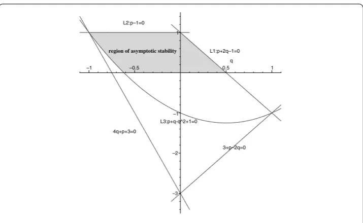
Figure 1 Region of asymptotic stability of system (1.1).

By the Jury’s conditions, the necessary and sufficient conditions for all eigenvalues of the characteristic equation lying inside the unit circle are:

⎧

We consider the following curves, which are the boundary curves of the region of asymp-totic stability shown in Figure :

⎧

OnL,L, respectivelyp= ,  which is impossible. We show in the following theorem occurrence of bifurcations on the boundary curvesL,L.

Theorem . For system (.) the following conditions holds:

() Flip bifurcation occurs when(p,q)∈L.

() Neimark-Sacker bifurcation occurs when(p,q)∈L.

Proof First, we show the existence of the flip bifurcation. Because (p,q)∈L, we have the characteristic equation:

which has eigenvaluesλ= –, λ,= (±

√

–q

 ). SoY = (, –, ) is an eigenvector ofH with corresponding eigenvalueλ = –, and  is not the eigenvalue. A straight forward calculation shows that:

Therefore by [, Th...], flip bifurcation occurs.

Now we show the existence of Neimark-Sacker bifurcation. Ifλ=eiθ_{is a root of}

Equa-tion (.), separating the real and imaginary parts, we have the following:

⎧ ⎨ ⎩

cosθ– (p+q)cosθ= –q,

sinθ– (p+q)sinθ= 

squaring and adding both equations, we have:

 – (p+q)– (p+q)cosθ=q

Therefore, Equation (.) has a unique pair of complex roots:

argλ= ,±π_,±_π,±π. Thusλk_{= , fork= , ,  and . On the other hand we have:} previous discussion, we obtain  <cosθ<

, hencecosθ= . If cos

_{θ+ cosθ– (p+q) –}

 = , then fromcosθ=q_–andp+q=q_{– , we see thatq=±,±}

, which corresponds top= , , –_, –_ that is impossible onL. So we have that, (d_dq|λ|)_|p+q–q_+== . Therefore, by the generic Neimark-Sacker bifurcation theorem [, ], Neimark-Sacker bifurcation occurs, that is, the system (.) has a unique closed invariant curve bifurcating from the

equilibriumX*.

4 Direction of the bifurcations

In the previous section, we have shown that system (.) undergoes a flip (period-doubling) bifurcation when (p,q)∈Land a Neimark-Sacker bifurcation when (p,q)∈Lat equilib-rium pointX*. In this section, by using the normal form method for discrete systems, as studied by Sacker, Kuznetsov and Wiggins, we shall study the direction of the two bifur-cations and stability of the bifurcating invariant curves. We can write system as:

Following the algorithms given in Kuznetsov [], the critical normal form coefficient

c(), that determines the nondegeneracy of the period-doubling bifurcation and the sta-bility of period-doubling cycle, is given by the following formula:

c() =  

v,C(w,w,w)– 

v,Bw, (H–I)–B(w,w). (.)

From the above relations we have:

⎧ ⎨ ⎩

v,B(w, (H–I)–_{B(w,w))= ,}

v,C(w,w,w)=f_{– p}()

and therefore:

c() = f

_()

( –p).

Applying the general theory for the direction of flip bifurcation and stability of period doubling cycle (see Wiggins [] or Kuznetsov []), we derive the following result:

Theorem . For system (.) flip bifurcation occurs in X*when p+ q= , and if f () > , the flip bifurcation is supercritical and if f () < , the flip bifurcation is subcritical.

Now, we are going to study the direction of the Neimark-Sacker bifurcation and the stability of the bifurcating invariant curve inX*_{. In the above section, we see thatHhas} simple eigenvalues on the unit circle:

λ,=e±iθ, θ=

arc cos+(_(p+_pq₊)_q–₎q

 .

Letαbe a complex eigenvector corresponding toeiθ_{andβbe a complex eigenvector of the}

transposed matrixHT_{correspondinge}–iθ_{,i.e. Hα=e}iθ_α,HT_β=e–iθ_{β. By computation} we obtain the following eigenvectors:

α=,eiθ_,eiθT_{, β=}

,–

q e

–iθ_,–

q e

–iθ

T .

Normalizeαwith respect toβsuch that:

β,α= ,

where·,·means the standard scalar product inC_{defined byβ,α=β}

α+βα+βα, we have:

α=,eiθ_,eiθT_,

β= 

q– e–iθ

Following the algorithms given in Kuznetsov [], the critical normal form coefficient

a(), that determines the nondegeneracy of the Neimark-Sacker bifurcation and allows us to predict the stability of bifurcating invariant curve, is given by the following formula:

a() =  Re

e–iθ_{β,C(α,α,α)+ β,Bα, (I–H)}–_B(α,α)

+β,Bα,eiθ_I–H–_B(α,α).

Furthermore in this case we have:

β,C(α,α,α)=f

_()(eiθ_{– e}iθ_+eiθ_{– )}

(q– eiθ₎ ,

β,Bα, (I–H)–B(α,α)= ,

β,Bα,eiθ_I–H–_B(α,α)

=–(f

_())_(eiθ_{– e}iθ_{– e}iθ_{+ e}iθ_–eiθ_{– )}

(q– eiθ_)(eiθ_–peiθ₎ .

Which yields the following formula fora():

a() =f

_()A

+ (f ())A (A

+B)

in which:

A=qcosθ–qpcosθ– cosθ+ pcosθ,

B=qsinθ–qpsinθ– sinθ+ psinθ,

A= q+ qp– p+

p– q– qp–  – pcosθ

+ – p–q–qp+qpcosθ

+ (pq– p– )cosθ+ (–pq+ )cosθ

+ (pq+ p)cosθ+

p–qpcosθ

+ pcosθ– pcosθ,

A= (qp+ p)cosθ– qpcosθcosθ

+ qcosθcosθ– cosθcosθ

+ pcosθcosθ+ qpsinθ

+ (qp– p+q)cosθ+ (q–  – p)cosθ

+ (p– q)cosθ+ (p+ q)cosθ

+ cosθ– qcosθ– cosθ+ cosθ– qp.

Theorem . For system (.), if p+q–q_{+  = hold, then a() < (respectively> )}

im-plies that a unique and stable (respectively, unstable) closed invariant curve bifurcates from X*_{, and the Neimark-Sacker bifurcation in X}*_{is supercritical (respectively, subcritical).}

5 Numerical simulations

In this section, we give numerical simulations to illustrate our theoretical analysis.

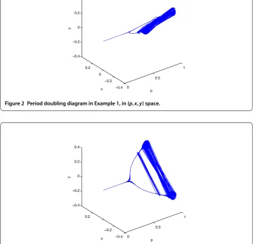
Example  Let p= _ andf(t) = _t+t_{. In this case q=} 

, c() =  and (p,q)∈L, therefore by Theorem . flip bifurcation occurs. Figures ,  and  show bifurcation dia-gram.

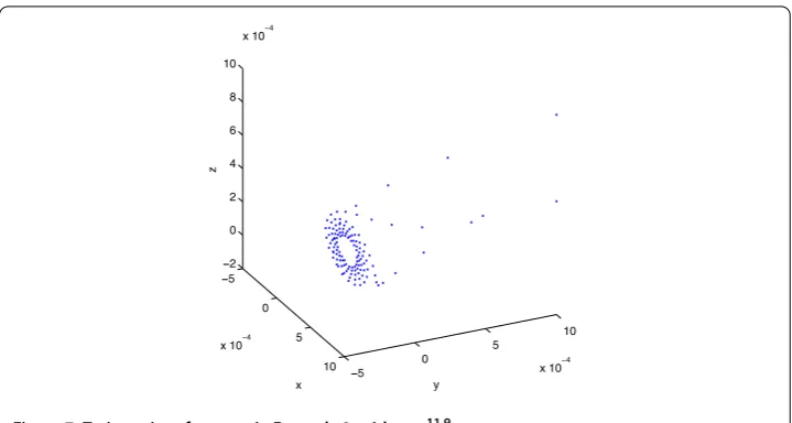
Example  Letp=_andf(t) = –_t+t_{. In this caseq= –}

,a() = –., and (p,q)∈

L, therefore by Theorem . Neimark-Sacker bifurcation occurs. Figures ,  and  show orbits of system whenp=_,p=_ andp=._, respectively.

Figure 2 Period doubling diagram in Example 1, in (p,x,y) space.

Figure 4 Period doubling diagram in Example 1, in (p,y,z) space.

Figure 5 Trajectories of system, in Example 2, withp= 9 25.

Figure 7 Trajectories of system, in Example 2, withp=11.9₂₅.

Competing interests

The authors declare that they have no competing interests.

Authors’ contributions

All authors carried out the proof. All authors conceived of the study, and participated in its design and coordination. All authors read and approved the final manuscript.

Acknowledgements

The authors would like to thank the referees for their useful comments.

Received: 9 March 2012 Accepted: 14 June 2012 Published: 16 July 2012

References

1. Eckaus, RS: The stability of dynamic models. Rev. Econ. Stat.39, 172-182 (1957) 2. Hicks, JR: A Contribution to the Theory of the Trade Cycle. Clarendon, Oxford (1965)

3. Dai, B, Zhang, N: Stability and global attractivity for a class of nonlinear delay difference equations. Discrete Dyn. Nat. Soc.3, 227-234 (2005)

4. Li, S, Zhang, W: Bifurcations in a second-order difference equation from macroeconomics. J. Differ. Equ. Appl.2, 365-374 (2007)

5. Sedaghat, H: A class of nonlinear second-order difference equations from macroeconomics. Nonlinear Anal.29, 593-603 (1997)

6. Sedaghat, H: Nonlinear Difference Equations: Theory with Applications to Social Science Models. Kluwer Academic, Dordrecht (2003)

7. Stuart, AM, Humphries, AR: Dynamical Systems and Numerical Analysis. Cambridge University Press, Cambridge (1998)

8. Kuznetsov, YA: Elements of Applied Bifurcation Theory. Springer, New York (1998)

9. Wiggins, S: Introduction to Applied Nonlinear Dynamical Systems and Chaos. Springer, New York (1990) 10. Sacker, RJ: On invariant surfaces and bifurcation of periodic solutions of ordinary differential equations. Technical

report IMM-NYU 333, New York University (1964)

11. Sacker, RJ, Von Bremen, HF: Bifurcation of maps and cycling in genetic systems. Fields Inst. Commun.42, 305-311 (2004)

doi:10.1186/1687-1847-2012-107