R E S E A R C H
Open Access
A robust beamformer design for underlay
cognitive radio networks using worst case
optimization
Uditha Lakmal Wijewardhana
1*, Marian Codreanu
1, Matti Latva-aho
1and Anthony Ephremides
2Abstract
We propose a robust beamforming design for underlay cognitive radio networks where multiple secondary
transmitters communicate with corresponding secondary receivers and coexist with a primary network. We consider a scenario where all transmitters have multiple antennas and all primary and secondary receivers are equipped with a single antenna. The main focus is to design the optimal transmit beamforming vectors for secondary transmitters that maximize the minimum of the received signal-to-interference-plus-noise ratios of the cognitive users. The
interference powers to the primary receivers are kept below a threshold to guarantee that the performance of the primary network does not degrade due to the secondary network. Imperfect channel state information (CSI) in all relevant channels are considered, and a bounded ellipsoidal uncertainty model is used to model the CSI errors. We recast the problem in the form of semidefinite program and an iterative algorithm based on the bisection method is proposed to achieve the optimal solution. Further, we propose upper and lower bounds for the optimal value of the considered problem, which provides better initialization for the algorithm. Numerical simulations are conducted to show the effectiveness of the proposed method against the non-robust design.
Keywords: Cognitive radio networks; Optimization; Robust beamforming design; Semidefinite programming (SDP); Semidefinite relaxation
1 Introduction
Scarcity of wireless spectrum is one of the major chal-lenges faced by the modern wireless communication industry. Due to rapid deployment of wireless services in the recent past and the fixed spectrum allocation pol-icy, the wireless spectrum has been increasingly crowded. On the other hand, according to the Federal Communi-cation Commissions and other regulatory bodies, most of the allocated spectrum is under utilized [1]. Therefore, the secondary usage of wireless spectrum has been pro-posed as a method to utilize more efficiently the wireless spectrum [1-4].
Cognitive radio networks (CRNs) [2-4] operate on this idea of the secondary usage of spectrum. Here, the sec-ondary network is allowed to opportunistically access the spectrum owned by the primary network provided that *Correspondence: [email protected]
1Centre for Wireless Communications, University of Oulu, P.O. Box 4500, Oulu 90014, Finland
Full list of author information is available at the end of the article
it does not degrade the performance of the primary net-work. Hence, there are two major challenges that should be addressed by a CRN. The first challenge is to maximize the performance of the users in the CRN as much as possi-ble. The second challenge is to guarantee the performance or the quality of service (QoS) of the primary network, which is the main constraint in a CRN. Specifically, in
underlayCRNs, the performance of the secondary (cog-nitive) users should be maximized while the maximum interference power to the primary users (PUs) should remain below a pre-specified threshold [4].
achieve a locally optimal solution and an alternative centralized algorithm has been proposed based on geo-metric programming and network duality. A game the-oretic approach for the same problem with a CRN that coexists with multiple PUs is presented in [6].
However, in practice, the channel vectors are estimated from training sequences and, inherently, this leads to imperfect estimation. These CSI estimation errors can greatly affect the performance of the network, result-ing in degradation in both primary and secondary users’ QoS. Such channel errors are usually modeled either by a bounded uncertainty model such as D-norm, polyhedron, ellipsoidal [10] or a stochastic error model [11].
Robust beamformer design with imperfect CSI has received a considerable attention recently. Usually, this problem is tackled by either worst-case optimization [12-27] or stochastic optimization [24,28]. In worst-case optimization (or maximin optimization), the uncertain parameters can take some given set of possible values, but without any known distribution. Then the optimiza-tion variables are designed in such a way that an objective value is maximized while guaranteeing the feasibility of the constraints over the given set of possible values of the parameters. This method has been applied to design the robust beamforming vectors for underlay CRNs in [20-26], where the channel errors are either norm bounded or bounded by ellipsoids. With the exception of [24] and [26], most of the abovementioned work consider a CRN where a single secondary transmitter (TX) co-exists with a primary network. The problem of maximizing the minimum signal-to-interference-plus-noise ratio (SINR) in an underlay CRN, where the transmitter communi-cates with multiple secondary receivers (RXs) is studied in [21]. An iterative solution has been proposed based on semidefinite relaxation [29], and if the solution is not rank-one, rank-one approximations [29] have to be used to achieve the beamforming vectors. For the same problem, a method to achieve a rank-one solution with some tol-erance is presented in [22]. Therefore, none of the above work guarantee the optimal solution of the problem of maximizing the minimum SINR in an underlay CRN.
The sum mean square error is minimized in [24] for an underlay MIMO ad hoc CRN constrained to individ-ual power budgets of secondary TXs, where the channel errors are bounded by Euclidean balls. There the authors have cast the problem as a semidefinite program (SDP) and solved iteratively via standard interior point methods to achieve a suboptimal solution for the problem. In [26], the same problem of minimizing the sum mean square error for an underlay MIMO ad hoc CRN subject to individual power budgets for the secondary TXs was con-sidered. A distributed solution was proposed under the assumption that secondary TXs have perfect CSI knowl-edge of the channels to the secondary RXs. Furthermore,
the SINR of an underlay MIMO secondary link is max-imized in [30] constrained to the power budget of the secondary TX under the same assumption that secondary TX has perfect CSI knowledge of the channel to the secondary RX.
The focus of this paper is to design the optimal robust beamforming vectors for the secondary TXs in a CRN that coexists with a primary network. We address the problem of maximizing the worst SINR of any secondary user sub-ject to interference constraints to primary network and individual power constraints. Further, we assume that the network controller has imperfect CSI knowledge and all relevant channel vectors may take any value within some pre-specified bounded uncertainty ellipsoids [10,14,17]. An equivalent reformulation of the problem is obtained, and then the S-procedure [31,32] is used to handle the non-convex quadratic constraints due to channel uncer-tainties. In particular, we replace each quadratic con-straint pair by a linear matrix inequality (LMI) for a fixed objective value by means of the S-lemma [18,21], which leads to a SDP. An iterative algorithm based on the bisec-tion method is proposed to solve the relaxed version (relaxed the non-convex rank constraints in the problem) of the reformulated problem. Finally, we show that the optimal solution for the original problem can be achieved by introducing a properly chosen objective function to the feasibility check step of the iterative algorithm.
As the main contribution, in this work, we show the abil-ity to handle CSI uncertainty in a multiple-input-single-output (MISO) communication network with interference temperature constraints. Further, we provide a rigorous proof for the tightness of SDP relaxation in worst SINR maximization problem in multi-cell downlink scenario with a single user per cell and subject to interference temperature constraints. Additionally, we show that the proposed solution approach can be extended to maximize the worst weighted SINR or, more generally, the worst among a set of increasing functions of each SINR.
Organization: Section 2 describes the network and the channel uncertainty models used in this paper. The prob-lem formulation for the worst-case scenario and a suit-able equivalent reformulation is presented in Section 3. In Section 4, the SDP-based solution is presented and an iterative algorithm is proposed to obtain the optimal beamforming vectors. Simulation results are presented in Section 5. Finally, we conclude the paper with Section 6.
denotes the transpose and (·)H denotes the Hermitian (conjugate transpose) operation for a vector or a matrix. W 0 andW 0 means thatWis positive semidefi-nite and positive defisemidefi-nite, respectively. Rank and the trace of a matrix are represented by Rank(W) and Trace(W), respectively. Modulus of a scalar is denoted by| · |and · denotes the Euclidean norm of a vector. The expectation of a random variable is denoted byE{·}. In addition,In
denotes then-dimensional identity matrix while0denotes an all-zero vector or matrix with appropriate dimen-sions. We denote the complex normal distribution with meanμand covarianceσ2byCN(μ,σ2). The distribution
T CN(μ,σ2,a,b)represents the truncated complex
nor-mal distribution with parametersμ,σ2,aandb(see [33], Chap. 4 in [34]). Finally, in an optimization problem, if
wis a variable, thenw denotes the optimal value or the optimal solution.
2 System model
We provide the detailed description of the considered sys-tem model in this section. Specifically, we describe the network model and the channel uncertainty model used throughout the paper.
2.1 Network model
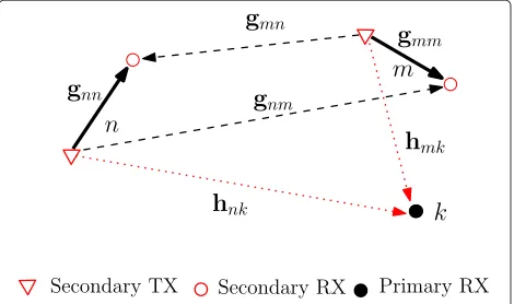
We consider an underlay CRN consisting of multiple transmitter-receiver pairs which coexists with a primary network. The network model is shown in Figure 1. The set of secondary links is denoted byN and we label them asn = 1,. . .,N. We use the same indexing for the sec-ondary transmitters and receivers, i.e., we refer to the transmitter (receiver) of the nth secondary link as the
nth secondary TX (RX). We consider a MISO downlink scenario and assume that each secondary TX (a base sta-tion) is equipped withntantennas to communicate with
its corresponding secondary RX (a mobile station). We
Figure 1System model.Underlay cognitive radio network with two secondary TX-RX pairs (N=2) coexists with a primary network consisting a single primary RX (K=1). Straight arrows show the desired channels and the dashed arrows show the interfering channels.
represent the set of all primary RXs byKand label them ask = 1,. . .,K. Further, we assume that all the primary and secondary RXs are equipped with a single antennaa.
We assume that all secondary TXs operate in the same frequency band as the primary network and use transmit beamforming to communicate with their corresponding secondary RXs. We further assume that a network con-troller decides the resource allocation and beamforming vectors for each secondary TX.
Single-stream beamforming transmission strategy is assumed and hence the signal transmitted by the nth secondary TX is given by
xn=wndn, (1)
wheredn denotes the (complex) information symbol and
wnis its associated beamforming vector. We assume that
the information symbols are independent, i.e.,E{dndHm} =
0 for all m = n,n,m ∈ N, and normalized such that
E{|dn|2} =1 for alln∈N. Therefore, the transmit power
of thenth secondary TX is given bywn2and it is
lim-ited byPmax, the maximum available transmit power, for
alln∈N.
We denote the channel vector from themth secondary TX to thenth secondary RX by gmn ∈ Cnt. The signal
received at thenth secondary RX can be written as
yn=gHnnwndn+ N
m=1 m=n
gH
mnwmdm+zn, (2)
where the first term is the signal of interest, the second term represents the interference from the secondary net-work andzn∈Cis the additive noise at thenth secondary
RX. We assume that the noise termznhas powerσn2and it
includes the receiver’s thermal noise and the interference from the primary network. Therefore, the instantaneous SINR at thenth secondary RX can be expressed as
SINRn=
gH
nnwn2
N
m=1 m=n
gH
mnwm2+σn2
. (3)
The interfering channel from thenth secondary TX to the
kth primary RX is denoted byhnk ∈ Cnt. Now, the total
interference power caused by the secondary network on thekth primary RX can be written as
Ik = N
n=1
hH
nkwn2, (4)
which should be limited by the interference thresholdIth
in order to guarantee the QoS of the primary network. 2.2 Channel uncertainty model
possible values. Specifically, we assume that the channel vectors,gmnandhnk for alln,m∈ N andk ∈ K, belong
to known ellipsoidal uncertainty sets.
We model the channel vector,gmn, from the mth
sec-ondary TX to thenth secondary RX as the sum of two components, i.e.,
gmn= ˆgmn+emn, (5)
where gˆmn ∈ Cnt denotes the estimated value at the
network controller and emn represents the
correspond-ing channel estimation error. It is assumed that emncan
take any value inside ant-dimensional complex ellipsoid.
Hence, the channel uncertainty set can be defined as
Emn(Qmn)=
emn:eHmnQmnemn≤1
, (6)
where Qmn is a complex Hermitian positive definite
matrix (Qmn0), assumed to be known, which
speci-fies the size and shape of the ellipsoid. For example, when Qmn =
1/ξmn2 I, the ellipsoidal channel error model (6) reduces toemn2 ≤ ξmn2 . This represents a ball
uncer-tainty region [35] with unceruncer-tainty radius ξmn. In this
model, ξmn = 0 implies that perfect CSI knowledge is
considered and withξmnthe channel uncertainty becomes
larger causing CSI knowledge to become imperfect [21]. We use the same uncertainty model for the channel vec-tor, hnk, from thenth secondary TX to thekth primary
RX, i.e.,
hnk = ˆhnk+ ˜enk, (7)
where hˆnk ∈ Cnt is the estimated value at the network
controller and e˜nk denotes the corresponding channel
estimation error. The ellipsoidal channel uncertainty set can be defined as
˜ Enk Q˜nk
=e˜nk :e˜nkHQ˜nke˜nk ≤1
, (8)
where Q˜nk 0 specifies the size and shape of the
uncertainty ellipsoid. 3 Problem formulation
Our objective is to maximize the performance of the CRN while satisfying the QoS requirements of the primary network. We consider the minimum SINR among all sec-ondary receivers as the performance indicator of the CRN and the interference received from the CRN as the QoS measurement for the primary network. Then the solution of the problem will guarantee a certain SINR for all sec-ondary RXs while the interference to all the RXs in the primary network will be lower than a predefined threshold
Ith. The mathematical formulation of the mentioned
prob-lem and a suitable equivalent reformulation is presented in this section.
3.1 Problem formulation
Now, with the channel uncertainty model above, we can re-write the instantaneous SINR at thenth secondary RX as
SINRn=
gˆnn+enn
Hw
n 2
N
m=1 m=n
gˆmn+emn
Hw
m 2
+σ2 n
, (9)
and the interference power, caused by the secondary net-work on thekth primary RX as
Ik = N
n=1
hˆnk+ ˜enkHwn
2. (10)
The resource allocation problem we address in this work is to optimize the transmit beamforming vectors in CRN,
{wn}Nn=1, to maximize the minimum SINR of the
sec-ondary RXs for given parameters Pmax and Ith. Due to
the CSI uncertainty, the beamfomer design should guar-antee a certain SINR for any channel error value inside the uncertainty region. Further, the design should keep the interference to the primary RXs below the threshold for all channel errors inside the uncertainty region to guarantee the performance of the primary network. This problem can be mathematically expressed as
maximize minn=1,...,Ninfemn∈Emn,m∈NSINRn
subject to sup˜e
nk∈ ˜Enk,n∈NIk≤Ith, k∈K
wn22≤Pmax n∈N,
(11)
where the optimization variables are wn,emn,e˜nk for
n,m ∈ N,k ∈ K. Note that SINRn depends onemnfor
allm ∈ N (see (9)) andIk depends one˜nk for alln ∈ N
(see (10)). In Problem (11), the infimum in the objective function and supremum in the first constraint are taken over all possible channel errors contained in the given uncertainty region.
3.2 An equivalent reformulation
p. 134 in [31]) (strictly speaking, this is a hypograph form, as Problem (11) is a maximization) asc
maximize γ
By introducing the new variables,
smn=
Problem (12) can be recast equivalently as
maximizeγ (15a)
where the optimization variables are γ and wn,emn,e˜nk,smn,Ink for alln,m ∈ N,k ∈ K. Note that
we have re-written 1st constraint in Problem (12) as two separate ones, i.e., (15b) and (15c). Furthermore, it is easy to show (e.g., by contradiction) that constraints (15c) and
(15e) are tight (i.e., they hold with equality at optimality). Hence, Problem (15) is an equivalent reformulation of Problem (12).
4 Optimal beamformer design
In this section, we propose an iterative algorithm to solve the equivalent Problem (15) and compute the optimal beamforming vectors for the underlay CRN.
4.1 Optimal solution and iterative algorithm
The outer productwnwHn in Problem (15) is a rank-one
positive semidefinite matrix. We introduce a new set of variables Wn = wnwHn for all n ∈ N. Then the
con-straints (15b), (15c), (15d) and (15f) become linear inWn,
andWnshould be rank one. Furthermore, we can see that
the constraint (15b) is quadratic inenn, constraint (15c) is
quadratic inemnand (15e) is quadratic ine˜nk. This
sug-gests that we can use the following lemma to recast these constraints in such a way that they become linear matrix inequalities (LMIs) for fixed value ofγ in Problem (15).
S-lemma[18,31,32]:Letibe a real valued function of
anl-dimensional complex vectory, defined as i(y)=yHAiy+2Re
following conditions are equivalent:
S1 :0(y)≥0for ally∈Clsuch that1(y)≤0. S2 : There existsλ≥0such that the following LMI is
feasible:
Consider the first constraint in Problem (15). It can be re-written as
should be satisfied. The existence of an enn for which
(17) holds strictly is obvious (e.g., enn = 0). Hence, we
can regard the left-hand sides of (16) and (17) as0(enn)
and 1(enn) in S-lemma. Then, according to S-lemma,
that satisfy (17) if there exists μnn ≥ 0 such that the
condition
nn
⎡
⎣ Wn Wngˆnn
ˆ gH
nnWn gˆHnnWngˆnn−γ
N m=1 m=n
smn+σn2
⎤⎦
+μnn
Qnn 0
0 −1
0, n∈N
(18) is satisfied.
Following the same procedure, it follows that the inequality (15c) is satisfied for all channel errorsemn ∈ Emnif there existsμmn≥0 such that
mn
−Wm −Wmgˆmn
−ˆgH
mnWm smn− ˆgHmnWmgˆmn
+μmn
Qmn 0
0 −1
0, m∈N\{n},n∈N
(19) is satisfied. Similarly, the inequality (15e) is satisfied for all channel errorse˜nk ∈ ˜Emnif there existsνnk ≥0 such that
nk
−Wn −Wnhˆnk
−ˆhH
nkWn Ink− ˆhHnkWnhˆnk
+νnk
˜
Qnk 0
0 −1
0, n∈N,k∈K
(20)
is satisfied.
Thus, we can rewrite Problem (15) equivalently as follows:
maximize γ
subject to nn0, n∈N
mn0, m∈N\{n},n∈N
nk 0, n∈N,k∈K
N
n=1Ink ≤Ith, k∈K
μmn≥0, n,m∈N
νnk ≥0, n∈N,k∈K
Wn0, n∈N
Trace(Wn)≤Pmax, n∈N
Rank(Wn)=1, n∈N,
(21)
where the optimization variables are γ and Wn,μmn,νnk,smn,Inkforn,m∈N,k∈K. Note that if the
rank constraints are neglected, Problem (21) can be easily solved using the bisection method (see p. 146 in [31]) which provides the optimal solution for Problem (21).
Specifically, for a fixedγ , the feasibility can be checked by solving the problem
P0(γ ): find {Wn,μmn,νnk,smn,Ink}n,m∈N,k∈K
subject to nn(γ )0, n∈N
mn0, m∈N\{n},n∈N
nk0, n∈N,k∈K
N
n=1Ink≤Ith, k∈K
μmn≥0, n,m∈N
νnk ≥0, n∈N,k∈K
Wn0, n∈N
Trace(Wn)≤Pmax, n∈N,
(22) where the optimization variables areWn,μmn,νnk,smn,Ink
for alln,m∈ N,k ∈K, using a standard SDP solver and the optimal solution is the maximum value ofγ for which Problem (22) is feasible.
However, it turns out that we can employ a simple trick to handle also the rank constraint of Problem (21). The procedure is based on replacing the dummy objective function in Problem (22) with the sum power minimiza-tion for the secondary network. Then the problem used to check the feasibility can be written as
P1(γ ): minimize Nn=1 Trace(Wn)
subject to constraints of P0(γ )
(23)
where the optimization variables areWn,μmn,νnk,smn,Ink
for alln,m ∈ N,k ∈ K. Clearly, Problem (22) is feasible if and only if Problem (23) is feasible (because they have the same set of constraints). Furthermore, the following proposition ensures that Problem (23) returns always a set of rank one matricesWn.
Proposition 1. If Problem (23) is feasible (for a givenγ), then the optimal matricesWn are always rank one, i.e., W
n=wnwnH for all n∈N.
Proof. The proof is presented in Appendix 1.
Note that for a given feasible value ofγ, Problem (22) can also have higher rank solutions but Problem (23) has only rank one solutions. The optimal beamforming vec-tors that maximize the minimum SINR can be found directly by eigen-decomposition ofWnfor alln∈N. This implies that the global optimal solution of the original Problem (11) is obtained.
In the bisection method, exactlylog2((γupp−γlow)/ )
iterations are required before the algorithm termi-nates (see p. 146 in [31]), whereγlowandγuppare the initial
lower and upper bounds for the optimal value. Hence, a good initialization can reduce the number of iterations required in the algorithm which leads to lower resource consumption. Therefore, in practice, it is highly beneficial to have good initial lower and upper bounds which are simple to obtain. Next, we describe an efficient method for finding lower and upper bounds (i.e.,γlowandγupp) to
initialize the above algorithm.
4.2 Initial lower bound
When a constraint in a maximization problem is modi-fied (perturbed) in such a way that it gets tightened, the optimal value of the perturbed problem is always a lower bound for the optimal value of the original problem (see pp. 249-251 in [31]). We use this fact to compute an efficient initial lower bound,γlow, for Algorithm 1.
Algorithm 1Robust cognitive beamforming via bisection method >0, initial lower and upper bounds for the optimal valueγlowandγupp.
repeat
1.γ :=γlow+γupp/2.
2. Solve the convex feasibilityProblemP1(γ ).
3.ifP1(γ )is feasible,γlow:=γ; elseγupp:=γ.
Consider the first constraint of Problem (15),
We introduce a new variable t, that should satisfy the inequality
Now, using (24) and (25), the constraint (15b) can be tightened as follows:
perturbed problem can be written as
maximize γ
where the optimization variables are γ,x and Vn,emn,e˜nk,umn,ynkfor alln,m∈N,k∈K.
Following the same method as in Section 4.1, using S-lemma to recast the quadratic constraints as LMIs, Problem (28) can be reformulated as follows:
where and the optimization variables are γ,x and Vn,μˇmn,νˇnk,umn,ynk for alln,m ∈ N,k ∈ K. Note that
the non-convex product terms γsmn (in Problem (21))
are not present in Problem (29). Hence, without the rank constraints the Problem (29) is convex (even whenγ is considered as a variable). Therefore, the relaxed prob-lem can be efficiently solved using SDP solvers such as SeDuMi [36] or SDPT3 [37].
Let us denote the optimal matricesVnfor Problem (29)
byVnfor alln∈N. Then a rank-one feasible solution for Problem (29) can be achieved by eigenvalue decomposi-tion as follows:
Vei
n =λmaxymaxyHmax, (33)
where λmaxis the maximum eigenvalue andymax
repre-sents the corresponding eigenvector of matrix Vn. The feasibility ofVein is proved in Appendix 2. Since the matri-ces Vein are feasible for the perturbed Problem (29), the corresponding objective value obtained by solving Prob-lem (29) is a lower bound for ProbProb-lem (15).
4.3 Initial upper bound
An upper bound for a maximization problem can be found by relaxing a constraint of the original problem. Specifically, here we relax the first constraint,
γ ≤ in Problem (12). Since the interference from themth sec-ondary TX to the nth secondary RX is a non-negative entity, i.e.,|(gˆmn+emn)Hwm|2≥0, the constraint (34) can
Now the perturbed Problem (12) with the relaxed con-straint can be written as
maximize γ
Following a similar approach as in sections 3.2 and 4.1, by introducing variables Wn = wnwHn,Ink = |(hˆnk +
˜ enk)Hw
n|2and using the S-lemma to recast the quadratic
constraints, Problem (36) can be reformulated as maximize γ Problem (37) can be efficiently solved using existing SDP solvers. Note that the non-convex product termsγsmn(in
version of Problem (37). Hence, the optimal solution of the relaxed problem also provides an upper bound for Problem (15).
4.4 Extension to a more general objective function Consider the resource allocation problem where the CRN is required to optimize the transmit beamforming vectors to maximize the worst weighted SINR or, more gener-ally the worst among a set of increasing functions of each SINR. Let fn be an increasing function of SINRn. Since
transmit power and primary interference constraints are inherited in underlay CRNs, for a bounded uncertainty in the channel errors, this problem can be mathematically expresseddas
maximize minn=1,...,Ninfemn∈Emn,m∈Nfn(SINRn)
subject to supe˜
nk∈ ˜Enk,n∈NIk≤Ith, k∈K
wn22≤Pmax n∈N,
(40) where the optimization variables are wn,emn,e˜nk for
n,m∈N,k∈K.
The function fn is an increasing function of SINRn;
hence,
inf emn∈Emn,m∈N
fn(SINRn)=fn
inf emn∈Emn,m∈N
SINRn
.
Therefore, the optimization Problem (40) can be equiva-lently written in the hypograph form (see p. 134 in [31]) as
maximize γ
subject to fn−1(γ )≤
gˆnn+enn
Hw
n 2
N
m=1 m=n|(ˆ
gmn+emn)Hwm|2+σn2
,
∀emn∈Emn, n∈N
N
n=1
hˆnk+ ˜enkHwn
2≤Ith,∀˜enk ∈ ˜Enk,
k∈Kwn22≤Pmax, n∈N,
(41) where the optimization variables are γ andwn,emn,e˜nk
for n,m ∈ N,k ∈ K. Problem (41) has the similar format as Problem (12), the only difference is thatγ in the first constraint of Problem (12) should be replaced by the evaluated function valuefn−1(γ )in Problem (41). Hence, following the similar steps as in sections 3.2 and 4, the Problem P1(γ ) can be modified according to the
new constraint. Then Problem (40) can be solved opti-mally by directly applying Algorithm 1 with the modified ProblemP1(γ )to check the feasibility.
5 Results and discussion
Numerical simulations are performed to validate and assess the performance of the proposed beamforming scheme. We consider a network model where two sec-ondary TX-RX pairs (N = 2) coexist in a primary network with two primary RXs (K = 2). We assume that each secondary TX is equipped with four anten-nas (nt = 4). Further, all complex entries of the
esti-mated channel vectors are independent and identically distributed (i.i.d) according toCN(0, 1). We assume that Qmn = ˜Qmk = (1/ξ2)Int for all n,m ∈ N,k ∈ K.
Thus, an estimation error can take any value inside a ball with radius ξ. We use a truncated normal distribution
T CN0,ξ2/9nt,−ξ/
√
2nt,+ξ/
√
2nt
(see [33], Chap. 4 in [34]) to generate each complex entry of the estimation errors. Additionally, we assume that σn2 = σ2 = 1 for alln ∈ N and the maximum available transmit power of a secondary TX is Pmax = 10σ2. To maintain the QoS
requirements for the primary network, we limit the max-imum allowable interference power from the secondary network in the order of the received noise power, i.e.,
Ith=σ2(=1).
We present results for both robust and non-robust beamforming designs for comparison. The robust beam-forming vectors are acquired directly following Algo-rithm 1 with tolerance = 10−2. For the non-robust case, the beamforming vectors are obtained based only on the estimated channels and ignoring the uncertainty. We follow the Algorithm 1 except that at step 2, we replace Problem (23) by the following one:
minimize Nn=1Trace(Wn)
subject to gˆHnnWngˆnn≥γ
N m=1 m=nˆ
gH
mnWmgˆmn+σn2
,
n∈N Nn=1hˆHnkWnhˆnk−Ith≤0, k∈K
Trace(Wn)−Pmax≤0, n∈N
Wn0, n∈N,
(42) where the optimization variables areWn for alln ∈ N.
The MATLAB toolbox CVX [38] is used to solve all the optimization problems, and there, the SDPs are solved using the SeDuMi solver.
−3 −2.5 −2 −1.5 −1 −0.5 0 0.5 0
0.1 0.2 0.3 0.4 0.5 0.6 0.7 0.8 0.9 1
Interference power at primary RX 1 [dB]
Prob (int. pow. <= abscissa)
ξ=0.1 (Robust)
ξ=0.2 (Robust)
ξ=0.3 (Robust)
ξ=0.4 (Robust)
ξ=0.5 (Robust) Non−robust design
ξ=0.1,0.2,0.3,0.4,0.5
Figure 2CDF of the interference due to the secondary network at a primary RX.Empirical CDF of the interference due to the secondary network at first primary RX for different values ofξ. A network with parametersnt=4,N=2 andK=2 is considered. The interference threshold for the primary network is 1 (0 dB). The empirical CDF is calculated over different channel errors for a fixed estimated channel realization.
when the CSI uncertainties are relatively small. Specifi-cally, with non-robust design, around 52%, 55%, 57%, 59% and 61% of the simulated channel errors exceed the inter-ference threshold of the primary network (Ith = 1) for
uncertainty ball radius of 0.1,0.2,0.3,0.4 and 0.5, respec-tively. On the other hand, for the proposed robust algo-rithm, the interference to the primary RX is always less than the threshold levele, which guarantees the required QoS of the primary network.
In Figure 3, we plot the empirical CDF of the interfer-ence due to the secondary network at first primary RX
−2.5 −2 −1.5 −1 −0.5 0 0.5 1
0 0.1 0.2 0.3 0.4 0.5 0.6 0.7 0.8 0.9 1
Interference power at primary RX 1 [dB]
Prob (int. pow. <= abscissa)
ξ=0.1 (Robust)
ξ=0.2 (Robust)
ξ=0.3 (Robust)
ξ=0.4 (Robust)
ξ=0.5 (Robust) Non−robust design
ξ=0.1,0.2,0.3,0.4,0.5
Figure 3CDF of the interference due to the secondary network at a primary RX.Empirical CDF of the interference due to the secondary network at first primary RX for different values ofξ. A network with parametersnt=4,N=2 andK=2 is considered. The interference threshold for the primary network is 1 (0 dB). The empirical CDF is calculated over different channel errors and over multiple estimated channel realizations.
for different values ofξ averaged over different estimated channel realizations. We generated 1,000 distinct esti-mated channel realizations and for each of them, 10,000 different channel errors are generated to calculate the empirical CDF. It can be seen that for more than half of the simulated cases, regardless the level of uncertainty, the non-robust solution exceeds the maximum interference threshold. On the other hand, the robust design guaran-tees the interference to the primary RX remain below the interference threshold (Ith = 1) for all simulated cases.
Moreover, it can be observed from Figures 2 and 3 that the variation in interference power becomes large with ξ. When the uncertainty region is small (i.e., small ξ), the beamformer can be designed to direct relatively sharp nulls towards primary RXs for all possible channel values within the uncertainty region. As the radiusξ increases, the range of possible channel values inside the uncer-tainty region increases as well and causes the nulls to become less focused. Hence, the interference power varies in a wider range for different channel errors inside the uncertainty region.
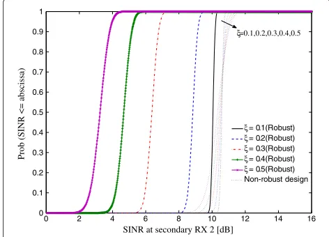
Figure 4 shows the empirical CDF of the received SINR at the second secondary RX for different values of ξ (i.e., the radius of uncertainty balls). We plot the SINR at the second secondary RX since it gives the minimum SINR for the considered value of the channel estimate. As in Figure 2, the empirical CDF is taken over 10,000 possible channel errors inside the uncertainty region. When the uncertainty region is small, the beamformer can be designed to direct relatively sharp nulls towards the primary RXs for all possible channel values within the uncertainty region. Hence, higher transmit powers can be allocated to the sharp beams towards the secondary RXs resulting in higher SINR values for smallerξ values. The
0 2 4 6 8 10 12 14 16
0 0.1 0.2 0.3 0.4 0.5 0.6 0.7 0.8 0.9 1
SINR at secondary RX 2 [dB]
Prob (SINR <= abscissa)
ξ= 0.1(Robust) ξ= 0.2(Robust) ξ= 0.3(Robust) ξ= 0.4(Robust) ξ= 0.5(Robust) Non-robust design ξ=0.1,0.2,0.3,0.4,0.5
ability of the secondary TXs to focus sharp beams towards the corresponding secondary RXs while simultaneously directing nulls towards other secondary and primary RXs reduces as the channel knowledge decreases (i.e., when ξ increases). Hence, the mean SINR reduces with the increase in the radius of uncertainty balls.
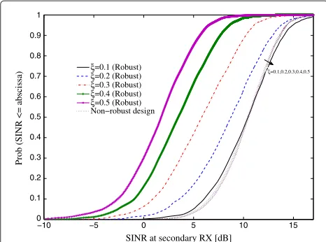
Figure 5 displays the empirical CDF of the received SINR at a specific secondary RX for different values ofξ, averaged over multiple estimated channels. As in Figure 3, we produced 1,000 different estimated channels, and for each of them, 10,000 different channel errors are gener-ated to calculate the empirical CDF. We can observe that the SINR performance of the robust design withξ = 0.1 is similar to the SINR performance of the non-robust design which is not able to guarantee the interference threshold. Thus, in average, our robust design provides a similar SINR performance for the secondary network as the non-robust design without exceeding the interference threshold of the primary network. Further, we notice a reduction in SINR when the uncertainty region increases. This is mainly due to the fact that the transmitter is not able to use all the available transmit power when the uncertainty region is large. This effect can be clearly seen in the next figure.
Figure 6 presents the transmit power variation at a specific secondary TX withξ (i.e., the radius of uncer-tainty balls). This figure is drawn using the same setup as in Figures 3 and 5. When the uncertainty region is small, since the nulls towards the primary RXs are sharp, higher transmit powers can be allocated to secondary TXs to achieve higher SINR values at secondary RXs. As ξ decreases from 0.3 to 0, we notice a rapid increase in the transmit power. On the other hand, when the uncertainty
−10 −5 0 5 10 15
0 0.1 0.2 0.3 0.4 0.5 0.6 0.7 0.8 0.9 1
SINR at secondary RX [dB]
Prob (SINR <= abscissa)
ξ=0.1 (Robust)
ξ=0.2 (Robust)
ξ=0.3 (Robust)
ξ=0.4 (Robust)
ξ=0.5 (Robust) Non−robust design
Figure 5CDF of the received SINR at a secondary RX.Empirical CDF of the received SINR at a secondary RX for different values ofξ. A network with parametersnt=4,N=2 andK=2 is considered. The empirical CDF is calculated over different channel errors and over multiple estimated channel realizations.
0 0.1 0.2 0.3 0.4 0.5 0.6 0.7 0.8 0.9 1
0 1 2 3 4 5 6 7 8 9 10
Radius of uncertainty sphere (ξ)
Tr
a
n
s
m
it
p
o
w
e
r
Figure 6Transmit power variation at a secondary TX.The transmit power variation at a secondary TX with respect to the radius of the uncertainty balls (ξ). A network with parametersnt=4,N=2 andK=2 is considered. Transmit power is averaged over 1,000 estimated channel realizations.
region is large, the beamformer design cannot focus sharp nulls towards primary RXs for all possible channel val-ues in the uncertainty region. Therefore, the transmitter has to decrease its transmit power to be able to guarantee the interference threshold for all possible channel values in the uncertainty region. Hence, forξ values greater than 0.5, the transmit power has become small.
Next, we illustrate the gain pattern variation of the beamforming vectors designed from non-robust and robust designs for different uncertainty regions (i.e., dif-ferent values ofξ). For illustration purposes, we consider a simple network model where a single secondary TX-RX pair (N = 1) coexist in a primary network with three primary RXs (K =3; see Figure 7). Further, we use a sim-ple line-of-sight model for the channels since the physical meaning of a beamforming pattern in a rich scattering environment is difficult to visualize with respect to the locations of the receivers. We model the estimated chan-nel vector from the secondary TX to secondary RX as g11 = g111,. . .,g11i ,. . .,gnt
11
T
, where the channel from antenna elementito secondary RX is given by [17]
gi11= √1
ntexp(2π
j/λ(xicosθ+yisinθ)), (43)
where (xi,yi) is the location of theith antenna element,
θ is the direction of the RX with respect to the direction of the antenna array andj = √−1. Similarly, we model the estimated channel vector from the secondary TX to the kth primary RX as h1k =
h11k,. . .,hi1k,. . .,hnt
1k
T
, where hi1k = √1
ntexp
2πj/λ(xicosθ +yisinθ)
gives the channel from antenna element i to thekth primary RX. We assume that the secondary TX is equipped with
0 0.5 1 1.5 2 0
0.2 0.4 0.6 0.8 1 1.2 1.4 1.6 1.8 2
SRx PRx STx
θ
Figure 7Network model for gain pattern comparison.Sample network. Secondary receiver at directionθ=45◦and primary receivers at directionsθ=60°,θ=90° andθ=120°. Network with parametersnt=10,N=1 andK=3. Antennas lie in a linear array λ/2 apart, centered at transmitter and along the directionθ=0°.
half-a-wavelength (λ/2) apart. Further, the antenna array is centered at the transmitter and lies along the direction θ = 0°. The secondary RX is located at directionθ =45° and the primary RXs are located at directionsθ = 60°, θ =90° andθ =120°.
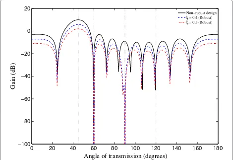
Figure 8 shows the gain patterns for the non-robust beamforming vector designed with estimated chan-nels and robust beamforming vectors designed with Algorithm 1. As expected, the gain reduces withξ, reduc-ing the SINR at the secondary RX since the TX have to decrease its transmit power to be able to guarantee the interference threshold for primary RXs. Further, as
0 20 40 60 80 100 120 140 160 180
−100 −80 −60 −40 −20 0 20
Angle of transmission (degrees)
Gain (dB)
Figure 8Gain pattern comparison.Gain pattern comparison for robust and non-robust beamforming designs. Network with parametersnt=10,N=1 andK=3. Antennas lie in a linear array λ/2 apart, centered at a transmitter and along the directionθ=0°. Vertical dotted lines represent the directional location of the receivers (secondary receiverθ=45°, primary receiversθ=60°, 90°, 120°).
ξ increases, we notice that the nulls around the angles at which the primary RXs are located become wider in order to protect the primary systemf. Therefore, Figure 8 validates the previous observations that as ξ increases the transmit power decreases reducing the SINR at sec-ondary RXs and nulls become wider around the angles at which the primary RXs are located to protect the pri-mary system, explaining the trade-off between secondary performance and the protection for the primary system. 6 Conclusion
We have proposed a method to design the optimal trans-mit beamformer vectors for an underlay cognitive radio network, which maximizes the minimum received SINRs of the cognitive users subject to primary users’ interfer-ence constraints. We have considered that the network controller has imperfect CSI knowledge in all relevant channels, and bounded ellipsoidal uncertainty model has been used to model the CSI errors. First, we have con-verted this highly untractable non-convex problem into a convex problem by means of semidefinite relaxation. Then, an iterative algorithm has been proposed based on the bisection method to solve the relaxed problem. Furthermore, we have provided a method to obtain the optimal solution for the original problem (i.e., non-relaxed problem) by introducing a properly chosen objective func-tion into the iterative algorithm. Finally, upper and lower bounds for the optimal value of the considered problem have been proposed, which provides better initialization for the algorithm. The simulation results show that the performance of the primary network is guaranteed by the proposed algorithm for any channel error within the considered uncertainty region. Furthermore, results show that for smaller uncertainty regions, the SINR perfor-mance of the proposed robust design is similar to that of the non-robust design.
Endnotes
aWe can apply the mathematical model of the proposed
network to more general network scenarios. As an example, we can consider a multi-cell network where the transmitters are base stations (BSs) equipped with multiple antennas that communicate with the single antenna mobile stations (MSs) using time-division-multiple-access. A BS transmits signals to a single MS at a given time instant and has per-transmission power constraints. Further, the multi-cell network is subject to some interference temperature constraints.
bWe assume that the equivalent channel and the power
of interference are perfectly known at each receiver.
cNote that the infimum and the supremum in
∀emn∈Emnand∀˜enk ∈ ˜Enkin the first and second
constraints of Problem (12), respectively. We can see that the variablesγ andwn,emn,e˜nkforn,m∈N,k∈Kare
optimal for Problem (12) if and only ifwn,emn,e˜nkfor
n,m∈N,k∈Kare optimal for Problem (11) and the first inequality constraint of Problem (12) holds with equality. Hence, the optimal solution of Problem (12) is equivalent to that of Problem (11).
dNote that in the worst weighted SINR case the
increasing functionsfn(SINRn)=ζnSINRnfor alln∈N,
whereζnis an arbitrary nonnegative weight associated
withnth secondary RX. Weightsζncan be used to
balance between user fairness and total throughput.
eNote that in worst-case robust optimization, the
beamforming vectors are designed to keep interference to the primary RXs below the threshold for all possible channel errors (irrespective of their probability of occurrence) inside the uncertainty region. In the simulations, each complex entry of the channel error vector is generated using a truncated Gaussian
distributionCN(0,ζ2)truncated at−3ζ and 3ζ(roughly speaking, this corresponds to 1% error outage), where ζ =ξ/3√2ntdenotes the standard deviation. The larger
value ofξimplies that the actual channel vector can be very far from the estimated value of the channel. Since in the considered simulation model, the probability of occurrence of the channel vectors which are far from the estimated value is small the probability of achieving interference close to the threshold is small.
fNote that in the non-robust design, there is no null
present atθ =90°. This is due to the fact that the beamforming design assumes perfect CSI at the secondary TX. Since the secondary TX knows the exact channel to the primary RX, even with this gain, the secondary TX can guarantee that the interference to the primary RX for that specific estimated channel is below the interference threshold.
Appendices Appendix 1
Proof of proposition 1
Let us rewrite Problem (23) as follows:
minimize Nn=1Trace(Wn) sponding dual variables for the constraints are shown in the rightmost column of Problem (44).
LetL(·)define the Lagrangian of Problem (44) and
nn=
value according to the properties of positive semidefinite matrices. Using the Karush-Kuhn-Tucker (KKT) condi-tions, gradient (∇), complimentary slackness (C.S.), pri-mal feasibility (P.F.) and dual feasibility (D.F.), we can write the following:
Further, we can observe for Problem (44) that the target minimum SINR
Now, we write the first-three term of (46) as toWn = 0which contradicts with (57). Therefore, the condition
nn=0, n∈N (60)
should be satisfied.
The rest of the proof follows from the proof of propo-sition 1 in [18] and we provide the details for the com-pleteness of the paper. First, we prove thatWn has rank one provided thatnnhas rank one. Then we prove that indeednnhas rank one.
Assume that nn has rank one and therefore it can be written as nn = vvH, where v ∈ Cnt+1.
, which has also rank one. So we can write
Using Sylvester’s rank inequality (see p. 211 in [39]) on (48) and with the help of (61), we can write following for rank ofWn: It follows from (57) and (62) that
RankWn=1. (63)
What remains is to prove thatnnindeed has rank one. First, we will show thatcnn > 0 andμnn > 0. From (47) and (55), we can write
TraceQnnAnn
≤cnn, n∈N. (64)
SinceQnn 0, by (45), (60) and (64), it is obvious that
cnn >0. We can see from (18) that whenμnn =0,nnis
not positive semidefinte because
By substituting (18) and (45) into (49), the following two equalities can be easily obtained:
W
adding to (66) result in
which is indeed a rank-one matrix. This concludes the proof.
Appendix 2
Proof of feasibility of eigenvalue approximation
Consider a positive definite matrix Y ∈ Hl with r =
Rank(Y). Then according to the eigenvalue decomposi-tion, we can write
Y=
Yis positive semidefinite, for any random vectorz∈Cl,
zHYz≥λ
1zHy1yH1z≥0. (71)
Here, the first inequality is achieved from the fact that all the eigenvalues are non-negative and the definition of positive semidefinite matrix gives the second inequality.
matricesVnfor alln∈N there exists aγ ≥0 such that the following conditions are satisfied:
Therefore, in order to show that the eigenvalue approx-imation is feasible, we should be able to find a γ ≥ 0 for the approximated beamforming vectors such that all above inequalities are satisfied.
Let the rank ofVnber, eigenvalues and the correspond-ing eigenvectors beλ1,n ≥ λ2,n ≥,. . .,≥ λr,n ≥ 0 and
y1,n,y2,n,. . .,yr,nrespectively for all n ∈ N. Then, using
the eigenvalue decomposition, the trace of the beamform-ing matrix can be written as
TrVn=
where the inequality is obtained using (72) and the fact that all eigenvalues are non-negative. Therefore, it can be easily shown from (74) that the condition (73f) is satisfied for the eigenvalue approximation.
Then from (71), for any error vectore˜nkwe can say that,
ˆ
This implies that the condition (73e) is satisfied with the approximation. Further, the same method can be applied to prove that the condition (73c) is also satisfied.
According to (71), in order to satisfy the condition (73a), the beamforming matrixVn should be rank one for all
n ∈ N, i.e., when the first inequality of (71) becomes an equality. But from the second inequality of (71), we can say that for any error vectorennthere exists someγnew, such
that
This concludes the proof and shows that we can find a γnew ≥0 for the eigenvalue approximation such that the
problem is feasible, but which will be a lower bound for the solution.
Competing interests
The authors declare that they have no competing interests.
Author details
1Centre for Wireless Communications, University of Oulu, P.O. Box 4500, Oulu
90014, Finland.2University of Maryland, College Park, MD 20742, USA.
Received: 06 August 2013 Accepted: 03 March 2014 Published: 12 March 2014
References
1. FCC, Spectrum policy task force report. Tech. Rep. TR 02–155 (2002). http://www.fcc.gov/sptf/reports.html. Accessed 15 March 2013 2. J Mitola III, Cognitive radio: an integrated agent architecture for software
defined radio. PhD thesis, Royal Institute of Technology, Sweden, 2000 3. S Haykin, Cognitive radio: brain-empowered wireless communications.
IEEE J. Selected Areas Commun.23(2), 201–220 (2005)
4. A Goldsmith, SA Jafar, I Maric, S Srinivasa, Breaking spectrum gridlock with cognitive radios: an information theoretic perspective. Proc. IEEE97(5), 894–914 (2009)
5. SJ Kim, GB Giannakis, Optimal resource allocation for MIMO ad hoc cognitive radio networks, inProceedings of the Annual Allerton Conference on Communications, Control, and Computing,23–26 September 2008 (Monticello, IL, 2008), pp. 39–45
6. G Scutari, DP Palomar, S Barbarossa, Competitive optimization of cognitive radio MIMO systems via game theory, inProceedings of the International Conference on Game Theory for Networks(Istanbul, Turkey, 2009), pp. 452–461
7. H Islam, YC Liang, A Hoang, Joint power control and beamforming for cognitive radio networks. IEEE Trans. Wireless Commun.7(7), 2415–2419 (2008)
8. L Zhang, R Zhang, YC Liang, Y Xin, HV Poor, On Gaussian MIMO BC-MAC duality with multiple transmit covariance constraints. IEEE Trans. Inf. Theory58(4), 2064–2078 (2012)
9. L Zhang, Y Xin, YC Liang, Weighted sum rate optimization for cognitive radio MIMO broadcast channels. IEEE Trans. Wireless Commun.8(6), 2950–2959 (2009)
10. K Yang, Y Wu, J Huang, X Wang, S Verdu, Distributed robust optimization for communication networks, inProceedings of the IEEE International Conference on Computer Communications,15–17 April 2008 (Phoenix, AZ, 2008), pp. 1157–1165
11. M Shenouda, TN Davidson, On the design of linear transceivers for multiuser systems with channel uncertainty. IEEE J. Selected Areas Commun.26(6), 1015–1024 (2008)
Speech, and Signal Processing,22–27 May 2011 (Prague, Czech Republic, 2011), pp. 3096–3099
13. SJ Kim, A Magnani, A Mutapcic, SP Boyd, ZQ Luo, Robust beamforming via worst-case SINR maximization. IEEE Trans. Signal Process.56(4), 1539–1547 (2008)
14. RG Lorenz, SP Boyd, Robust minimum variance beamforming. IEEE Trans. Signal Process.53(5), 1684–1696 (2005)
15. E Björnson, G Zheng, M Bengtsson, B Ottersten, Robust monotonic optimization framework for Multicell MISO systems. IEEE Trans. Signal Process.60(5), 2508–2523 (2012)
16. E Björnson, E Jorswieck, Optimal resource allocation in coordinated multi-cell systems. Foundations Trends Commun. Inf. Theory9(2-3), 111–381 (2013)
17. A Mutapcic, SJ Kim, S Boyd, A Tractable Method for Robust Downlink Beamforming in Wireless Communications, inProceedings of the Annual Asilomar Conference on Signals, Systems and Computers,4–7 November 2007 (Pacific Grove, CA, 2007), pp. 1224–1228
18. C Shen, TH Chang, KY Wang, Z Qiu, CY Chi, Distributed robust multicell coordinated beamforming with imperfect CSI: an ADMM Approach. IEEE Trans. Signal Process.60(6), 2988–3003 (2012)
19. SA Vorobyov, AB Gershman, ZQ Luo, Robust adaptive beamforming using worst-case performance optimization: a solution to the signal mismatch problem. IEEE Trans. Signal Process.51(2), 313–324 (2003)
20. F Wang, W Wang, Robust beamforming and power control for multiuser cognitive radio network, inProceedings of the IEEE Global
Telecommunication Conference,6–10 December 2010 (Miami, FL, 2010), pp. 1–5
21. G Zheng, KK Wong, B Ottersten, Robust cognitive beamforming with bounded channel uncertainties. IEEE Trans. Signal Process.57(12), 4871–4881 (2009)
22. MF Hanif, PJ Smith, M Alouini, SINR balancing in the downlink of cognitive radio networks with imperfect channel knowledge, inProceedings of the IEEE International Conference on Cognitive Radio Oriented Wireless Networks and Communications,9–11 June 2010 (Cannes, France, 2010), pp. 1–5 23. I Wajid, M Pesavento, YC Eldar, A Gershman, Robust downlink
beamforming for cognitive radio networks, inProceedings of the IEEE Global Telecommunication Conference,6–10 December 2010 (Miami, FL, 2010), pp. 1–5
24. EA Gharavol, Y Liang, K Mouthaan, Robust linear transceiver design in MIMO ad hoc cognitive radio networks with imperfect channel state information. IEEE Trans. Wireless Commun.10(5), 1448–1457 (2011) 25. Y Huang, Q Li, WK Ma, S Zhang, Robust multicast beamforming for
spectrum sharing-based cognitive radios. IEEE Trans. Signal Process.60, 527–533 (2012)
26. Y Zhang, ED Anese, GB Giannakis, Distributed optimal beamformers for cognitive radios robust to channel uncertainties. IEEE Trans. Signal Process.60(12), 6495–6508 (2012)
27. L Zhang, YC Liang, Y Xin, HV Poor, Robust cognitive beamforming with partial channel state information. IEEE Trans. Wireless Commun.8(8), 4143–4153 (2009)
28. G Zheng, S Ma, KK Wong, TS Ng, Robust beamforming in cognitive radio. IEEE Trans. Wireless Commun.9(2), 570–576 (2010)
29. ZQ Luo, WK Ma, AMC So, Y Ye, S Zhang, Semidefinite relaxation of quadratic optimization problems. IEEE Signal Process. Mag.27(3), 20–34 (2010)
30. YJ Zhang, AMC So, Optimal spectrum sharing in MIMO cognitive radio networks via semidefinite programming. IEEE J. Selected Areas Commun.
29(2), 362–373 (2011)
31. S Boyd, L Vandenberghe,Convex Optimization. (Cambridge University Press, Cambridge, 2004)
32. UT Jönsson, A Lecture on the S-procedure (2001). http://www.math.kth. se/~ulfj/5B5746/Lecture.ps. Accessed 12 January 2013
33. CP Robert, Simulation of truncated normal variables. Springer J. Stat. Comput.5(2), 121–125 (1995)
34. DJ Olive, Applied robust statistics. Preprint M-02-006 (2008). http:// lagrange.math.siu.edu/Olive/ol-bookp.htm. Accessed 1 March 2013 35. M Botros, TN Davidson, Convex conic formulations of robust downlink
precoder designs with quality of service constraints. IEEE J. Selected Top. Signal Process.1(4), 714–724 (2007)
36. I Polik, SeDuMi (2010). http://sedumi.ie.lehigh.edu/. Accessed 25 January 2013
37. KC Toh, MJ Todd, RH Tütüncü, SDPT3 – A Matlab software package for semidefinite programming, Version 1.3. Optimization Methods Softw.
11(1-4), 545–581 (1999)
38. CVX Research I, CVX: Matlab Software for Disciplined Convex Programming (2012). http://cvxr.com/cvx. Accessed 25 January 2013 39. CD Meyer,Matrix Analysis and Applied Linear Algebra. (Society for Industrial
and Applied Mathematics, Philadelphia, PA, 2000)
doi:10.1186/1687-1499-2014-37
Cite this article as:Wijewardhanaet al.:A robust beamformer design for
underlay cognitive radio networks using worst case optimization.EURASIP
Journal on Wireless Communications and Networking20142014:37.
Submit your manuscript to a
journal and benefi t from:
7Convenient online submission
7Rigorous peer review
7Immediate publication on acceptance
7Open access: articles freely available online
7High visibility within the fi eld
7Retaining the copyright to your article