The roles of conic sections and elliptic curves in the global dynamics of a class of planar systems of rational difference equations

R E S E A R C H

Open Access

The roles of conic sections and elliptic curves

in the global dynamics of a class of planar

systems of rational difference equations

Sukanya Basu

*_{Correspondence:}

[email protected] Department of Mathematics, Central Michigan University, Mount Pleasant, MI 48859, USA

Abstract

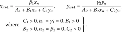
Consider the class of planar systems of first-order rational difference equations

xn+1=α_A1+_1+Bβ₁1_xx_nn₊+_Cγ₁1_yy_nn

yn+1=α_A2+_2+Bβ₂2_xx_nn₊+_Cγ₂2_yy_nn

, n= 0, 1, 2,. . ., (x0,y0)∈R, ()

whereR={(x,y)∈[0,∞)2:Ai+Bix+Ciy= 0,i= 1, 2}, and the parameters are nonnegative and such that both terms in the right-hand side of (1) are nonlinear. In this paper, we prove the following discretized Poincaré-Bendixson theorem for the class of systems (1).

If the map associated to system (1) is bounded, then the following statements are true:

(i) Ifbothequilibrium curves of (1) arereducible conics, then every solution converges to one of up to four equilibria.

(ii) Ifexactly oneequilibrium curve of (1) is areducible conic, then every solution converges to one of up to two equilibria.

(iii) Ifbothequilibrium curves of (1) areirreducible conics, then every solution converges to one of up to three equilibria or to a unique minimal period-two solution which occurs as the intersection of twoelliptic curves.

In particular, system (1) cannot exhibit chaos when its associated map is bounded. Moreover, we show that if both equilibrium curves of (1) are reducible conics and the map associated to system (1) is unbounded, then every solution converges to one of up to infinitely many equilibria or to (0,∞) or (∞, 0).

MSC: 39A05; 39A11

Keywords: difference equation; rational; global behavior; equilibrium; orbit; globally attracting; coordinatewise monotone; equilibrium curve; reducible conic; irreducible conic; minimal period-two solution

1 Introduction and main theorem

Consider the system of first-order rational difference equations with nonnegative param-eters

xn+=_Aα_₊+β_B_xx_nn₊+_Cγ_y_yn_n

yn+=_Aα_₊+_Bβ_xx_nn₊+_Cγ_y_yn_n

, n= , , , . . . , (x,y)∈R, ()

whereR={(x,y)∈[,∞):Aix+Biy+Ci= ,i= , }, and the parameters are nonnega-tive and such that both terms in the right-hand side of () are nonlinear. The class of sys-tems () has been widely studied in recent years when the RHS is both linear and nonlinear. For example, general solutions of planar linear discrete systems with constant coefficients and weak delays were studied by Diblík and Halfarová in [] and []. Global behavior of so-lutions and basins of attraction of equilibria for special nonlinear cases of system () called competitive and anticompetitive systems were studied by authors such as Basu, Merino and Kulenović in [] and [–]. Patterns of boundedness of nonlinear cases of system () were studied by Ladaset al.in [–]. More general results for system () as well its lower-and higher-dimensional counterparts were obtained by, for example, Basu lower-and Merino in [], by Stević, Diblíket al.in [–], and by Ladaset al.in [].

The class of systems () was proposed in all its generality by Camouziset al.in []. A number of open problems regarding () were also mentioned in the latter. Our goal in this paper is to give a complete qualitative description of the global behavior of solu-tions to all systems () whose maps are bounded and thus provide answers to many of the open problems in []. For example, we present the global dynamics of the system la-beled (, ) in open problem  and the competitive system lala-beled (, ) in open lem  in []. We also give the global analysis of the following  systems in open prob-lem  which may be competitive in some range of its parameters but nowhere cooperative: (,l) and (,l) withl∈ {, , , , , }, (, ), (, ), and (,l), (,l) with

l∈ {, , , }. The eight systems (, ), (, ), (, ), (, ), (, ), (, ), (, ) and (, ) from open problem , which may be competitive in a certain region of parameters, cooperative in another region of parameters and neither competitive nor cooperative in a third region of parameters, are also analyzed in this paper.

We also look at the four systems (, ), (, ), (, ) and (, ) from open prob-lem  which may be cooperative in some range of parameters but nowhere competitive. In addition, we present the global dynamics of a number of cases of system () from open problem  which are neither competitive nor cooperative in any parameter region along with many additional cases that were not mentioned in [], namely, cases (k,l) withk>l. In all, we give the global dynamics of all  cases of nonlinear system () for which both members of the system are bounded along with  cases for which one or more members of the system are unbounded. We also show that for all of these cases, for which there exists a unique nonnegative equilibrium and no minimal period-two solutions, local sta-bility of the equilibrium implies global attractivity. Thus we provide the answer to open problem . in [] for the cases mentioned above.

Members of the class of systems () have proven to be very useful for modeling purposes in biological sciences (see [–]). For example, the Leslie-Gower model from theoretical ecology is the two-species competition model

xn+=_+cb_x_nx₊n_cyn

yn+=_+cb_x_ny₊n_cyn

, n= , , . . . , (x,y)∈[,∞)×[,∞), (LG)

stan-dard linearization techniques. Moreover, this system is competitive (see [–]). So, it is somewhat easier to analyze global behavior of its solutions.

Unfortunately, most members of class () do not possess either of these two nice proper-ties of simple formulas for their equilibria and competitiveness. Another challenge faced in the study of class () is the presence of a large number of parameters (twelve), which makes algebraic computations involving standard linearization techniques very compli-cated. One also needs to analyze a large number of individual cases (, cases) of () which is neither practical nor efficient. Finally, members of this class tend to possess mul-tiple equilibria and minimal period-two solutions possibly at the same time. Due to these difficulties, the global dynamics of members of this class remains largely unanalyzed to date. In [], Merino and the author introduced a new geometrical technique to analyze local and global behavior of solutions to a special case of system (E), the modified Leslie-Gower model

xn+=_+cb_x_nx₊n_cyn+h

yn+=_+cb_x_ny₊n_cyn+h

, n= , , . . . , (x,y)∈[,∞)×[,∞). (LG-)

The technique is based on the analysis of slopes ofequilibrium curvesof the system which are defined as follows. IfT(x,y) := (T(x,y),T(x,y)) is a map associated to the system, then the two equilibrium curves of the system are respectively given by the formulasT(x,y) =x

andT(x,y) =y. Thus these curves are analogous to nullclines in differential equations and their intersection points are precisely the equilibria of the system. This method was then used to establish a connection between the number of equilibria of the system and their local stability. The authors were then able to use this result along with the results proved by Kulenović and Merino in [] to give a complete qualitative description of the global dynamics of (LG-). Also in [], Merino and the author introduced another new method to analyze global behavior of solutions to two classes of second-order rational difference equations which are not competitive. The goal of this paper is to apply these two new techniques to analyze global behavior of solutions to the more general family of first-order planar systems of rational difference equations () with nonnegative parameters. In particular, a geometrical criterion is presented to classify a large number of cases of system (E) into subclasses exhibiting similar global dynamics. LetP⊂R_{be the set of} nonnegative parameters (α,β, . . .) such that the RHS terms in system () are nonlinear. The main theorem of this paper is as follows.

Theorem  If the map associated to system()is bounded with parameters inP,then the

following is true:

(i) If both equilibrium curves of ()are reducible conics,that is,if i. C(Cα–Aγ) +γ(Cβ–Bγ) = ,and

ii. B(Bα–Aβ) +β(Bγ–Cβ) = ,

then system()has at least one and at most four equilibria.Every solution converges to an equilibrium.

(ii) If exactly one equilibrium curve of ()is a reducible conic,that is,if either i. C(Cα–Aγ) +γ(Cβ–Bγ) = ,or

ii. B(Bα–Aβ) +β(Bγ–Cβ) = ,

(iii) If both equilibrium curves of ()are irreducible conics,that is,if i. C(Cα–Aγ) +γ(Cβ–Bγ)= ,and

ii. B(Bα–Aβ) +β(Bγ–Cβ)= ,

then system()has at least one and at most three equilibria.Every solution converges to an equilibrium or to a unique minimal period-two solution which occurs as the intersection of two elliptic curves.

Moreover,if both equilibrium curves of ()are reducible conics and the map associated

to system()is unbounded,then every solution converges to one of up to infinitely many

equilibria or to(,∞)or(∞, ).

We treat the three cases of Theorem  as three smaller theorems and devote three sep-arate sections of the paper to their respective proofs. What makes case (i) of Theorem  relatively easy to analyze is the fact that the mapTassociated to system () is coordinate-wise monotone in this case. Hence the global dynamics of its orbits is relatively easy to track. In case (ii), the mapTis monotone in only one coordinate. Here the global dynam-ics of its orbits is a bit more complicated. However, the most complicated dynamdynam-ics occurs in case (iii) where the mapTis not monotone in any coordinate. In this case, the bounded setB:= [L,U]×[L,U] containing the solutions to system () can be subdivided into five regions of coordinatewise monotonicity based on the relative positions of a pair of vertical linesx=Kandx=Kand a pair of horizontal linesy=Landy=Lin the setB as shown below:

(a) {K,K} ∩[L,U] =φand{L,L} ∩[L,U] =φ,

(b) EitherK∈[L,U]orL∈[L,U], andK∈/[L,U],L∈/[L,U],

(c) EitherK∈[L,U]orL∈[L,U], andK∈/[L,U],L∈/[L,U],

(d) K,L∈[L,U]orK,L∈[L,U],

(e) K,K∈[L,U]orL,L∈[L,U].

HereKandLdepend on the parameter valuesα,β, . . . ,B,C, whileKandLdepend on the parameter valuesα,β, . . . ,B,C. To prove case (iii), we will show that there exists a nested sequence of invariant attracting boxes{Bi}∞i= with the property thatB∗=

Bi satisfies exactly one of the following:

(i) B∗= (x,y).

(ii) There exist equilibria(x,y_) se(x,y) se(x,y)such that(x,y)and(x,y)lie

at the north-west and south-east corners ofB∗, respectively, and(x,y_)lies in its interior.

(iii) There exist minimal period-two solutions(p,q) se(x,y) se(r,s)such that(p,q)

and(r,s)lie at the north-west and south-east corners ofB∗, respectively, and(x,y)

lies in its interior.

In case (i), it is clear that the unique equilibrium (x,y) is globally attracting. In case (ii), we show that the local stability of the equilibria is determined by the slopes of the equilibrium curves at these equilibria. In case (iii), we prove that system () has a unique minimal period-two solution by looking at intersections of certain elliptic curves. We then use these results to give global stability results for the two cases.

This paper is organized as follows. In Section , we look at the admissible parameter re-gions and initial conditions for system (). In Section , we define the notions ofsouth-east

order,competitive mapsandequilibrium curvesof system (). In Section , we look at

In Section , we look at regions of coordinatewise monotonicity for the mapT(x,y). Sec-tions  and  respectively deal with the case where both equilibrium curves of system () are reducible conics and the case where exactly one of them is a reducible conic. Sec-tions .-. respectively deal with the number of nonnegative equilibria, local stability of equilibria, existence and uniqueness of minimal period-two solutions, and global behavior of solutions of system () when both equilibrium curves are irreducible conics.

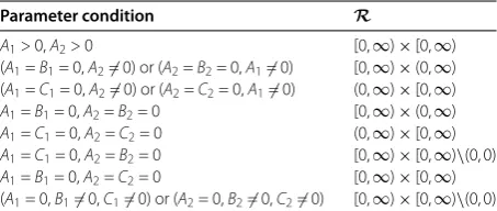
2 Parameter regions and initial conditions

In this section, we look at conditions that the parametersα,β, . . . ,BandCof system () must satisfy in order to be included in the setPintroduced in Theorem  in the previous section. In particular, note that the parameters inPmust satisfy the following inequalities:

Bi+Ci>  one of the members of system () becomes linear. Since we are interested in studying non-linear rational systems of difference equations belonging to class (), we will ignore these cases. Next, note that ifαi+βi+γi=  fori=  or , then at least one of the members of system () becomes trivial causing the latter to reduce to a difference equation. Since we are interested in studying systems of difference equations belonging to class (), we will ignore these cases as well. Similarly, ifAi=Bi=αi=βi=  orAi=Ci=αi=γi=  for

i∈ {, }, then at least one of the members of system () becomes constant, and we have the same situation as before, which we want to avoid.

The assumption that each of the twelve parametersαi,βi,γi,Ai,BiandCifori∈ {, } can be zero or positive and the inequalities in hypotheses () imply that fori=  there are _{–  =  ways to choose the numerator of the first member of system () excluding the} trivial case α=β=γ= . Similarly, there are seven ways to choose the denominator. Thus there are × =  ways to choose the first member of system (). Out of these, only  –  =  choices satisfy the last two inequalities in hypotheses (). Similarly, there are  choices for the second member of system (). In all, there are × = , ways to choose systems belonging to class (). Moreover, the initial condition (x,y)∈Rmust be chosen according to Table  in order to avoid division by zero.

Table 1 RegionsRof initial conditions

3 Important definitions

In this section, we provide some key definitions which we will frequently refer to through-out this paper. LetT be the map associated with system (), that is,

T(x,y) :=

α+βx+γy

A+Bx+Cy

, α+βx+γy

A+Bx+Cy

:=T(x,y),T(x,y).

LetTandTbe the coordinate functions ofT, that is,

T(x,y) = α+βx+γy

A+Bx+Cy

and T(x,y) = α+βx+γy

A+Bx+Cy .

Then system () can be written as

xn+

yn+

=

T(xn,yn)

T(xn,yn)

=T

xn

yn

. ()

Definition  For a given choice of parameters inP, we say that system () is bounded if the associated mapT is bounded,i.e., if there exist nonnegative constantsc,C,cand

Csuch that

c≤T(x,y)≤C,

c≤T(x,y)≤C.

Definition  The south-east order seonRis defined as follows:

(x,y) se(x,y) ⇐⇒ x<x and y>y.

Definition  A continuous mapT:R→Ris said to be competitive if it is monotone with respect to the south-east ordering se.

Remark One can easily check that the Jacobian of a competitive map satisfies the sign structure+ –_{– +}.

Definition  The equilibrium curvesEandEof system () are the sets

E:=

(x,y)∈R:x=T(x,y), E:=

(x,y)∈R:y=T(x,y).

Note thatEandEarelociof conic sections:

E:Bx+Cxy+ (A–β)x–γy–α= ,

E:Cy+Bxy+ (A–γ)y–βx–α= .

()

i. C(Cα–Aγ) +γ(Cβ–Bγ)= ,

ii. B(Bα–Aβ) +β(Bγ–Cβ)= .

Moreover, sinceC≥ andB≥,EandEcannot be ellipses. In this paper, we con-sider three separate cases, namely, the cases where (i) bothEandEare reducible conics, (ii) exactly one ofEandEis a reducible conic, and (iii) bothEandEare irreducible conics.

4 Bounded cases of system (1)

In this section, we look atbounded casesof system (), that is, special cases of system () for which all solutions with nonnegative/positive initial conditions are bounded. These cases have the property that their associated maps are bounded. They are obtained by setting one or more of the twelve nonnegative parametersα,β,γ,A,B,C,α,β,γ,

A,BandCto zero in system () and have been studied in great detail by Ladaset al. in, for example, [, ] and [], to name a few. For a more complete list of important work done in analyzing the boundedness of a large number of special cases of system () by Ladaset al., the reader is referred to references [–, , –]. Such systems have been referred to as having boundedness characterization (B, B) in these papers. In particular, explicit formulas for many of these systems were given in Appendices  and  of reference [].

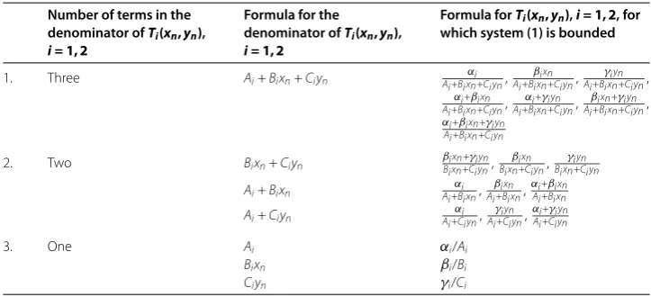
In this section, we show that there are at least  bounded nonlinear cases of system (). We also give explicit formulas for all of these  cases. This result is important because it shows that there are enough bounded nonlinear cases of system () (at least  cases!) to warrant the study conducted in this paper. It is stated next. Denote the expressions on the RHS of system () byT(xn,yn) andT(xn,yn) respectively as shown below:

xn+=T(xn,yn),

yn+=T(xn,yn).

()

Theorem  If the functions T(xn,yn)and T(xn,yn)in the RHS of ()have one of the

formulas given below,then system()is bounded:

Table 2 Some formulas forT1(xn,yn) andT2(xn,yn) for which system (1) is bounded

Thus there are at leastbounded cases of system()of whichcases are nonlinear.

Proof To see the proof of part (a) of the theorem, observe that ifT(xn,yn) has the first

formula in the RHS of Table  case  withi= , then one can respectively choose lower and upper boundsLandUforT(xn,yn) as follows:

This idea extends to the other formulas in case  as well. For the last formula in case , one can do even better with the choice of bounds as shown below:

L:= min{α,β,γ}

A similar idea can be used to find bounds for the formulas in case  of Table . In case , the bounds are trivial since the formulas are constant to begin with. Moreover, ifT(xn,yn) has one of the formulas in Table  withi= , then one can find lower and upper boundsL andUfor it in the same manner as before. In addition, ifT(xn,yn) has the first formula

One can similarly findL andU for the second case in (). In the third case, one can choose

The fourth case in () is similar. In the fifth case, one can choose

The bounds for the last case in () can be found in a similar manner. The formulas in () are almost identical to the formulas in () withA,βandxnrespectively replaced byA,γ andyn. Hence their lower and upper boundsLandUcan be found in a similar fashion as in (). It follows from the previous discussion that there are  +  +  +  +  =  bounded formulas forT(xn,yn) and another  bounded formulas forT(xn,yn) in cases (i)-(iv) of Table  of part (a). In all, there are × =  bounded cases of system  in part (a) and × =  bounded cases each in parts (b) and (c). This gives a total of  + () =  bounded cases of system  from parts (a), (b) and (c). Moreover, there are × =  ways to pairT(xn,yn) andT(xn,yn) so that both of them are constant in the RHS of (): three choices for T(xn,yn) from Table  case  wheni=  combined with three choices for

T(xn,yn) from Table  case  wheni= . In addition, the first two formulas in both parts (b) and (c) of the theorem are linear. They can be combined to give × =  cases where

T(xn,yn) andT(xn,yn) are both linear in the RHS of (). Finally, there are × =  ways each to respectively combine the two linear formulas in parts (b) and (c) with those in Table  case  so that the RHS of () is a combination of a linear formula and a constant formula. This gives a total of  +  =  cases. To conclude, there are  +  +  =  linear or constant cases out of the  bounded cases we originally identified above, which leaves us with  –  =  bounded nonlinear cases of system ().

The goal of this paper is to give a complete qualitative description of the global behav-ior of solutions to all bounded nonlinear cases of system () including the  bounded nonlinear cases mentioned in Theorem  above.

5 Regions of coordinatewise monotonicity for the mapT

When both equilibrium curves are irreducible conics, the map T(x,y) associated to bounded system () is not coordinatewise monotone throughout its bounded domain of definition. In this subsection, we will identify regions of coordinatewise monotonicity of the mapT(x,y). These regions will play a crucial role in determining the global behavior of solutions to system () when both equilibrium curves are irreducible conics.

Lemma  The following statements are true:

(i) IfBγ–Cβ= ,then the partial derivatives of the functionsT(x,y)are continuous

on(,∞)_{and have constant sign on the setB.}

(ii) IfBγ–Cβ= ,then the partial derivatives of the functionsT(x,y)are

continuous on(,∞)and have constant sign on the setB.

Proof We give the proof of part (i). The proof of part (ii) is similar and we skip it. Note

that by hypotheses (), B+C > . First, suppose B =  and C = . Solving forγ inBγ–Cβ=  and substituting in ∂∂xT(x,y) and

∂

∂yT(x,y), we get that

∂

∂xT(x,y) = – Bα–Aβ

(A+Bx+Cy) and

∂

∂yT(x,y) = –

C(Bα–Aβ)

B(A+Bx+Cy). When B =  and C = , the

hypothe-sis implies thatβ= . In this case,DT(x,y) =  andDT(x,y) = –C_B(Bα–Aβ)

(A+Cy) . Finally,

when B =  andC= , one must have γ=  and hence DT(x,y) = –B_(Aα_₊–_BA_xβ₎ and

DT(x,y) = . Clearly, in all three cases the partial derivatives ofT(x,y) have constant

sign on the setB.

Lemma  Suppose Biγi–Ciβi= for i= , .The functions Ti(x,y),i= , ,have continuous

For the rest of this paper, we will need to refer to the relative positions ofKiandLiwhere the partial derivatives ofTi(x,y) change sign fori= , . The explicit formulas forKiand

Li fori= ,  are given in the following definition. Their relative positions according to different parameter regions are shown in the Appendix for convenience.

Definition  IfBγ–Cβ=  and Bγ–Cβ= , set

Lemma  The following statements are true:

(i) K∈[,∞)if and only ifL∈/ [,∞);

(ii) K∈[,∞)if and only ifL∈/ [,∞).

Proof We give the proof of part (i). The proof of part (ii) is similar and we skip it. Suppose

K∈[,∞)andL∈ [,∞). Then the parametersα,β,γ,A,B,C,α,β,γ,A,

BandCmust satisfy one of the following:

(a) Bγ–Cβ> ,Bα–Aβ< ,Cα–Aγ≥;

(b) Bγ–Cβ< ,Bα–Aβ≥,Cα–Aγ< .

Note thatA,BandCmust be strictly positive in this case in order to avoid contradicting the inequalities in (a) and (b). Hence one can respectively rewrite the inequalities in (a) and (b) as

6 When bothE1andE2are reducible conics

In this section, we discuss global behavior of solutions when both equilibrium curvesE andEare reducible conics, that is, bothEandEare pairs of parallel, perpendicular or transversal (non-perpendicular) lines. In order for this to be true, bothE andE must have one of the forms given below:

Remark The missing parameters in the equations in () are assumed to be nonnegative. Also note that:

(i) In cases (a),EandEeach belong to a pair of parallel lines. The corresponding

members of system()have the forms

xn+=

(ii) In cases (b),EandEeach belong to a pair of perpendicular lines. The

corresponding members of system()look like

xn+=

(iii) In cases (c),EandEbelong to a pair of non-perpendicular transversal lines each.

The corresponding members of system()have the forms

xn+=

Note that the first equation in (i) involvingxn+actually consists of six separate equations corresponding to three cases each forAi=  andAi= . These three cases are: (a)α= ,

β= , (b)α= ,β=  and (c)α= ,β= . The same is true for the second equation in (i) involvingyn+. Similarly, the two equations in (ii) each consist of two separate equations, namely, the one withAi=  and the one withAi=  fori= , . The same is true of (iii).

Thus this section establishes global behavior of solutions of system () when its members are combinations of any of the  +  +  =  forms forxn+with any of the ten forms for

yn+given in (i)-(iii) of the last remark. This gives rise to  explicit planar systems of first-order rational difference equations with positive parameters. It is a direct consequence of Table  in Theorem  that the equations in (i) and (iii) are bounded while the equations in (ii) are unbounded. Thus there are a total of ( + )×( + ) =  bounded systems out of the  systems. Moreover, if both members of () have the forms given in (iii) and, in addition,A>  andA> , then the resulting system is the well-known Leslie-Gower model from theoretical ecology whose global dynamics was analyzed by Cushinget al.in []. The main theorem of this section is the following.

Theorem  If system()is bounded and if both its equilibrium curves Eand Eare

re-ducible conics,that is,if

i. C(Cα–Aγ) +γ(Cβ–Bγ) = ,and

ii. B(Bα–Aβ) +β(Bγ–Cβ) = ,

then it has at least one and at most four equilibria.Every solution converges to an

equilib-rium.

6.1 Number of nonnegative equilibria

The main theorem of this subsection is the following.

Theorem  If system()is bounded and satisfies the hypotheses of Theorem,then it has

at least one and at most four equilibria in [,∞).Moreover,

(a) If there exists one equilibrium,then it must be(, )or an interior equilibrium. (b) If there exist two equilibria,then they must include an axis equilibrium.

(c) If there exist three equilibria,then they must consist of(, )and an equilibrium on each axis.

(d) If there exist four equilibria,then they must consist of(, ),an equilibrium on each axis and an interior equilibrium.

Proof It follows from the discussion preceding this subsection thatEmust have one of

the following forms:

(a) Bx+ (A–β)x–α= , whereC=γ= ,

(b) x(Cy+A–β) = , whereC> ,α=γ= ,B= ,

(c) x(Bx+Cy+A–β) = , whereC> ,α=γ= ,B> .

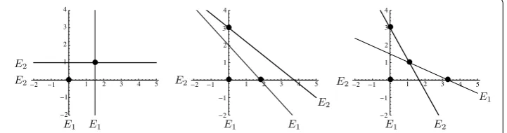
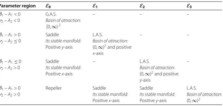
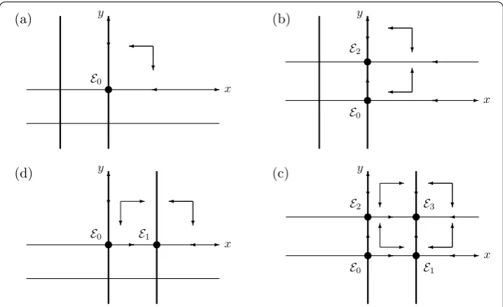
Case (a) represents a pair of vertical lines. Case (b) represents a pair of perpendicular lines withx=  as one of them. This case is unbounded by the discussion in the previous section. Case (c) represents a pair consisting of the vertical linex=  and a line with a negative slope in thexy-plane. Similarly, the reducible conicE must consist of a pair of horizontal lines, a pair of perpendicular lines withx=  ory=  as a member or a pair consisting of the horizontal line y=  and a line with a negative slope in the xy-plane. If none of the four lines coincide, then clearly they must intersect in at least one and at most four points in [,∞). Some possibilities are shown in Figure . If one or more lines representingE coincide with one or more lines representingE, thenE andE must intersect in infinitely many points in [,∞).

Next we discuss the global behavior of solutions to system () when it satisfies the hy-potheses of Theorem .

6.2 Global behavior of solutions

In this section, we present the proof of Theorem . In order to do so in a manageable way, we break up the statement of Theorem  into six smaller theorems based upon whether the equilibrium curves of system () consist of two parallel lines, two perpendicular lines, two transversal lines or some mix of the three (refer to cases (i)-(iii) at the start of Section ).

In particular, we give the explicit proof for the case where both equilibrium curves are parallel lines and state the remaining five theorems, Theorems -, in the Appendix at the end of this paper to avoid unnecessary repetition.

First, we present a definition and a lemma which will be required for the proof of the theorem mentioned above.

Definition  Recall the definition of equilibrium curves from Section :

E=

(x,y)∈R:x=f(x,y),

E=

(x,y)∈R_:y=f (x,y)

.

Consider the mapT= (f,f) associated to system () restricted to the set (,∞). Set

R(–, –) :=(x,y)∈(,∞)_:f

(x,y) <x,f(x,y) <y

,

R(–, +) :=(x,y)∈(,∞):f(x,y) <x,f(x,y) >y,

R(+, –) :=(x,y)∈(,∞):f(x,y) >x,f(x,y) <y,

R(+, +) :=(x,y)∈(,∞):f(x,y) >x,f(x,y) >y

.

Let (x,y) be an equilibrium of system (). Denote byQ,= , , ,  the four regions

Q(x,y) :=(x,y)∈(,∞):x<x,y<y,

Q(x,y) :=(x,y)∈(,∞):x>x,y<y,

Q(x,y) :=(x,y)∈(,∞):x>x,y>y,

Q(x,y) :=(x,y)∈(,∞):x<x,y>y.

Lemma  If the map T: [,∞)→[,∞)is competitive and possesses an interior

equi-librium(x,y)which satisfies

Q(x,y) =R(–, –), Q(x,y) =R(+, –),

Q(x,y) =R(+, +), Q(x,y) =R(–, +),

()

then(x,y)is globally asymptotically stable.

Proof By the hypotheses and the fact that any competitive mapT(x,y) preserves the

south-east order se, we have

(x,y)∈Q(x,y) ⇒ (x,y) seT(x,y) seT(x,y) se· · · seTn(x,y)

se· · · se(x,y),

(x,y)∈Q(x,y) ⇒ (x,y) se· · · seTn(x,y) se· · · seT(x,y)

In both cases, it follows thatTn_{(x,y)→(x,y). Also, note that sinceT is competitive in} (,∞)_{, and hence inQ(x,y) = [x,U]×[y,U], one has}

min

(x,y)∈Q(x,y)

f(x,y) =f(x,U) and min

(x,y)∈Q(x,y)

f(x,y) =f(U,y). ()

Since the point (x,U) lies on the linef(x,y) =x, one hasf(x,U) =x. Similarly, the point (U,y) lies on the linef(x,y) =yand hencef(U,y) =y. It follows from this and () that

Q(x,y) is invariant. By a similar reasoning, one can show thatQ(x,y) is invariant. This and hypotheses () imply that

(x,y)∈Q(x,y) ⇒ (x,y) <· · ·<Tn(x,y) <· · ·<T(x,y) <T(x,y) < (x,y),

(x,y)∈Q(x,y) ⇒ (x,y) <T(x,y) <T(x,y) <· · ·<Tn(x,y) <· · ·< (x,y).

Hence we haveTn_{(x,y)→(x,y) in both these cases.}

Our next theorem gives the global behavior of solutions when both equilibrium curves

EandEof system () are pairs of parallel lines. It is as follows.

Theorem  If the graphs of Eand Eare the pairs of parallel lines

E=

(x,y)∈R:Bx+ (A–β)x–α= 

,

E=

(x,y)∈R:Cy+ (A–γ)y–α= 

,

()

then the nonnegative equilibria of system()and their basins of attraction must satisfy the

following:

(i) Ifα= andα= ,then the unique equilibriumEis globally asymptotically stable.

(ii) Ifα= andα= ,then

• Ifβ–A≤,then the unique equilibriumEis globally asymptotically stable.

• Ifβ–A> ,thenEis a saddle point with the nonnegativey-axis as its stable

manifold.Eis LAS and attracts all solutions with initial conditions in(,∞)

or on the positivex-axis. (iii) Ifα= andα= ,then

• Ifγ–A≤,then the unique equilibriumEis globally asymptotically stable.

• Ifγ–A> ,thenEis a saddle point with the nonnegativex-axis as its stable

manifold.Eis LAS and attracts all solutions with initial conditions in(,∞)

or on the positivey-axis.

(iv) Ifα= andα= ,then the nonnegative equilibria of system()and their basins of

attraction must satisfy Table.

Proof First, supposeα=  andα=  in (). ThenEandEare given by the lines

x=β–A+

(β–A)+ αB B

and

y=γ–A+

Table 3 Global dynamics forα1= 0 andα2= 0 whenE1andE2are pairs of parallel lines

in [,∞). Clearly, they intersect at the unique equilibrium

(x,y) = is competitive and hence the unique equilibrium (x,y) is a global attractor by a result of Kulenović and Merino in []. Next, supposeα=  andα=  in (). ThenEandEare

C ). By Lemma ,Eattracts every solution with initial condition

in (,∞)_{or on the positivex-axis. Moreover, sinceT}_{(x,y) is competitive, it is easy to} check that

(, ) seT(, ) se· · · seTn(, ) seTn(,y) seE,

E seTn(,y) seTn(,U) se· · · seT(,U) se(,U).

Hence we haveTn_{(, )→EandT}n_{(,U)→E. As a result,T}n_{(,y)→Efor  <y<} U. ThusEis a saddle equilibrium with the nonnegativey-axis as its stable manifold.

The proof of the caseα=  andα=  in () is similar to the previous case and we skip it. Finally, supposeα=  andα=  in (). In this case,EandEare given by the lines

E: :x= , :x=

β–A

B ,

E: ˆ:y= , ˆ:y=

γ–A

C .

Ifβ–A≤ andγ–A≤, then,ˆ⊂(,∞)and the unique equilibriumE= (, ) is globally asymptotically stable by Lemma .

If β–A ≤ and γ –A > , then  ⊂(,∞) and ˆ⊂ (,∞). Hence E and E= (,γ–A

C ) are the only equilibria present. Note that in this case,Q(E) =R(–, –) and

Q(E) =R(–, +). Also, the dynamics of solutions with initial conditions along the positive x- andy-axes can be determined in the same way as in the proof of the caseα=  and

α= . The result follows from this and Lemma .

Ifβ–A>  andγ–A≤, then⊂(,∞)andˆ⊂(,∞). Hence the only equi-libria present areEandE= (β–A

B , ). This case is symmetric to the previous case and

has an almost identical proof.

Finally, ifβ–A>  andγ–A> , then,ˆ⊂(,∞)and hence all four equilibria E,E,EandE= (β–A

B ,

γ–A

C ) are present. In this case, global attractivity ofEin (,∞)



is guaranteed by Lemma . The proofs of the facts thatE,Eare saddle equilibria with the

x- andy-axes as their stable manifolds, respectively, and thatEis a repeller follow directly from analyzing the dynamics of solutions with initial conditions along the positivex- and

y-axes as shown in the proof of the caseα=  andα= . The four cases are shown in

Figure .

7 When exactly one ofE1andE2is an irreducible conic

In this section, we look at the case where exactly one of the equilibrium curvesEandE of system () is an irreducible conic and the mapT associated to system () is bounded. Note that this case corresponds toEandEbeing combinations of pairs of parallel lines, pairs of transversal non-perpendicular lines, parabolas and hyperbolas. The cases where

EorEis a pair of perpendicular lines are unbounded and hence not of interest to us in this paper. Thus there are ×( + )×( – ) =  bounded members and the rest are unbounded. The next theorem is the main theorem of this section and is as follows.

Theorem  If system()is bounded and if exactly one of its equilibrium curves Eand E

is a reducible conic,that is,if either

i. C(Cα–Aγ) +γ(Cβ–Bγ) = ,or

ii. B(Bα–Aβ) +β(Bγ–Cβ) = ,

then system()has at least one and at most two equilibria.Every solution converges to an

equilibrium.

The proof of the number of equilibria is given in the next theorem. To see that every solution converges to an equilibrium, observe that in this case, exactly one member of system () has one of the formulas given in (i)-(iii) of the previous section. Hence ex-actly one of the coordinates of the mapT(x,y) is monotone. Thus one can use a mix of the techniques already introduced in the previous section for reducible conics along with some new techniques that will be introduced in the next section for irreducible conics to prove global convergence results for this case. We skip the proofs to avoid unnecessary repetition.

Theorem  If system()is bounded and satisfies the hypotheses of Theorem,then it has

at least one and at most two equilibria in[,∞).Moreover,

(a) If there exists one equilibrium,then it may be an axis equilibrium or an interior equilibrium.

(b) If there exist two equilibria,then they must include an axis equilibrium and an interior equilibrium.

(c) The set of equilibrium points must be linearly ordered by ne.

Proof First, suppose thatEis an irreducible conic andEis a reducible conic. Then our

discussion at the start of this section implies thatEmust have one of the following forms:

(a) Bx+ (A–β)x–γy–α= , whereC= ,γ> ;

(b) Bx+Cxy+ (A–β)x–γy–α= , whereC> ,α+γ> .

In the first case,Erepresents a parabola that opens upwards and hasx-intercepts of op-posite signs ifα> , and a zerox-intercept ifα= . In the second case,Erepresents a hyperbola which hasx-intercepts of opposite signs ifα> , and a zerox-intercept if

Figure 3 The dots represent equilibria whenE1is an irreducible conic andE2is a reducible conic.

8 When bothE1andE2are irreducible conics

The main theorem of this section is the following.

Theorem  If system()is bounded and if both its equilibrium curves Eand Eare

irre-ducible conics,that is,if

i. C(Cα–Aγ) +γ(Cβ–Bγ)= ,and

ii. B(Bα–Aβ) +β(Bγ–Cβ)= ,

then system()has at least one and at most three equilibria.Every solution converges to an

equilibrium or to a unique minimal period-two solution which occurs as the intersection of

two elliptic curves.

We present the proof of Theorem  at the end of Section .. But first we present the number of nonnegative equilibria, local stability of equilibria, existence and uniqueness of minimal period-two solutions, and the global behavior of solutions to system () in Sections .-., respectively.

8.1 Number of nonnegative equilibria

We start this section by presenting a lemma which will help us establish bounds on the number of nonnegative equilibria of system () when both its equilibrium curves are irre-ducible conics.

Lemma  If the equilibrium curves Eand Eare irreducible conics,then all branches of

the sets

E=

(x,y)∈R:Bx+Cxy+ (A–β)x–γy–α= 

,

E=

(x,y)∈R:Cy+Bxy+ (A–γ)y–βx–α= 

are the graphs of monotone functions of one variable on an invariant attracting setB:=

[m,M]×[m,M]for system().In particular,

(i) IfC= andB= ,then the graphs ofEandEare parabolas with positive slopes

inB.

(ii) IfC> orB> ,then the graphs ofEandEare respectively hyperbolas whose

slopes inBhave signs as given in the last two columns of Table.The expression ‘+

or–’ implies an exclusive or.

Proof First, we look at the proof of part (i). It is easy to see that whenC=  andB= , the

Table 4 Signs of slopes ofE1andE2inBwhenC1> 0 orB2> 0

Moreover,Emust havex-intercepts of opposite signs ifα>  and a zerox-intercept if

α= . Similarly,Emust havey-intercepts of opposite signs ifα>  and a zeroy-intercept

ifα= . ThusEandEmust have positive slopes in [,∞)and hence in the setB. Next, we look at the proof of part (ii) whereC>  orB> . We give the proof for the slopes ofE. The proof for the slopes ofEis similar and we skip it. Note thatEcan be given explicitly as a function ofx:

E: y(x) =

C with a negative slope. It also hasx-intercepts of opposite signs when

α> ,

∂y has constant sign which is opposite to that of

∂T

∂x in all cases except for cases (iii) and (viii). In all such cases, observe that

∂T

C and is an increasing function ofx. Similarly, if

Figure 4 The arrows indicate types of coordinatewise monotonicity ofT1(x,y) in case (iii).

First, supposeK<_Cγ_. For all points (x,y)∈Bwithx<K,

minT(x,y) = lim x→K

y→∞

α+βx+γy

A+Bx+Cy = γ

C .

Moreover, for all points (x,y)∈Bwithx>K,

maxT(x,y) = lim

x→K

y→∞

α+βx+γy

A+Bx+Cy = γ

C .

Since an equilibrium (x,y) of system () is a fixed point that lies on the curveE, it fol-lows thatxmust satisfyK<x<_Cγ_. HenceEmust lie in the regionx<_Cγ_ and must be an increasing function ofx. One can similarly argue that ifK>_Cγ_, thenEmust be a de-creasing function ofx. Note that the caseK=γ_C_ cannot exist. Indeed, if it did, then the previous analysis would imply that the equilibrium (x,y) must lie on the linex=K=_Cγ_. But this is impossible since this line is a vertical asymptote for the curveEwhich contains the point (x,y). In case (viii), one can use a similar proof to show that ifK<_Cγ_, thenEis a decreasing function ofxand ifK>_Cγ_, thenEis an increasing function ofx. Corollary  The following statements are true.

i. The graph ofEis a decreasing function of a single variable inBif and only if

∂

∂yT(x,y) < .

ii. The graph ofEis a decreasing function of a single variable inBif and only if

∂

∂xT(x,y) < .

The next theorem establishes bounds on the number of nonnegative equilibria of sys-tem ().

Theorem  If both Eand Eare irreducible conics,then system()has at least one and

at most three equilibria in[,∞).In particular,

(a) IfEorEis a parabola,then either there exists a unique interior equilibrium or

there exist two equilibria,namely,(, )and an interior equilibrium which are linearly ordered by ne.

(b) If bothEandEare hyperbolas,then there exist between one and three equilibria all

of which are interior equilibria linearly ordered by se.

Proof From the proof of part (i) of Lemma , it follows that whenEandEare parabolas,

then note thatEcan be given explicitly as a function ofx:

C with a negative slope. It also hasx-intercepts of opposite signs when

α> 

must be increasing in the former case and decreasing in the latter case. Similarly, ifEis a parabola, then one can show that it must lie either in the regiony< β

B or in the region

y> β

B but not both. Also, it must be increasing in the former case and decreasing in the

latter case. It follows from this that ifEis a parabola andEis a hyperbola orvice versa, then the two must intersect in at most two points in [,∞)including (, ) and an inte-rior point. Moreover, if bothEandEare hyperbolas such that one or both of them are increasing in [,∞), then the opposite signs of their slopes/concavities guarantee that they must intersect in at most two points in [,∞)including (, ) and an interior point. Now suppose bothEandEare hyperbolas with decreasing branches in [,∞). It is a consequence of Bézout’s theorem (Theorem ., Chapter III in []) that the hyperbolas

EandEgiven in () must intersect in at most four points. Thus system () must have at most four equilibrium points. We claim that up to three of these four equilibrium points must lie inB. To see this, denote withQ(a,b),= , , ,  the four regionsQ(a,b) :=

can be given explicitly as functions ofx:

E:y(x) =

B is a horizontal asymptote ofE, it follows from

the decreasing characters ofy(x) andy–(x) that (c,y(c)) must lie inQ(γ

C,

β

B). When

C= , one can show that the equalities in () are still true and the conclusion follows from this. Some possible scenarios are shown in Figure .

8.2 Local stability of equilibria

Figure 5 The dots represent equilibria when bothE1andE2are irreducible conics.

we show that the local stability of the equilibria is determined by the slopes ofEandE at these equilibria. In Theorem , we present local stability results when bothE andE have negative slopes, and in Theorem , we do the same when at least one of them has a positive slope. We start out by giving a preliminary result on the equilibrium curves (sets) of system (). It is a generalization of Theorem  in [] and has weaker hypotheses than the latter. It also extends the latter to include the complex eigenvalues case and will be useful for proving Theorems  and .

Theorem  Let R be a subset ofR_{with a nonempty interior,and let T= (f,g) :R→R be}

a map of class Cp_{for some p≥.Suppose that T has a fixed point(x,y)∈intR such that}

a:=fx(x,y), b:=fy(x,y), c:=gx(x,y), d:=gy(x,y)

satisfy|a|< and|d|< .Let E,Ebe theequilibrium sets

E:=

(x,y) :x=f(x,y) and E:=

(x,y) :y=g(x,y). ()

Then

i. There exists a neighborhoodI⊂RofxandJ⊂Rofysuch that the setsE∩(I×J)

andE∩(I×J)are the graphs of classCpfunctionsy(x)andy(x)forx∈I.

ii. The eigenvaluesλandλof the Jacobian matrix ofTat(x,y)satisfy:

(a) Ifλ,λare real and equal,then– <λ,λ< .

(b) Ifλ,λare real and distinct withλ<λ,then– <λandλ< .Furthermore,

b= and

sign( +λ) =sign( +a+d+ad–bc) ()

and

sign( –λ) =

–sign(y_(x) –y_(x)) ifb< ,

sign(y_(x) –y_(x)) ifb> . ()

(c) Ifλandλare complex numbers,then

Proof

i. The existence ofIandJand of smooth functionsy(x)andy(x)defined inIas in the statement of the theorem is guaranteed by the hypotheses and the implicit function theorem. Moreover, whenfy(x,y)= , one has

y_(x) =  –fx(x,y)

fy(x,y)

and y_(x) = gx(x,y)  –gy(x,y)

, x∈I. ()

Note thatfy(x,y)= since otherwise one would havefx(x,y) = in()upon

rewriting the first expression asfy(x,y)y(x) =  –fx(x,y)and thusa:=fx(x,y) = ,

contradicting one of the hypotheses of the theorem. ii. The characteristic polynomial of the Jacobian ofT,

p(λ) =λ– (a+d)λ+ (ad–bc), ()

hasλandλas its roots. Ifλ=λ=λ, then the hypotheses– <a< and– <d< 

and the sum-of-roots relation for quadratic functions applied to()imply

– < λ=a+d<  ⇒ – <λ< ,

which proves (a). Now, supposeλ,λare real and distinct withλ<λ. Since – <a+d=λ+λ< , the larger rootλmust satisfy– <λand the smaller rootλ

must satisfyλ< . Moreover, the remark following()in part i gives that

b:=fy(x,y)= . To see the proof of(), note that in(), we have

p(–) =  + (a+d) +ad–bc= (– –λ)(– –λ). Since– <λfrom above, it follows

thatp(–) > if and only if– –λ< , that is, if and only if +λ> . Next note that

from(), we have

y_(x) –y_(x) = –a

b –

c

 –d=

 – (a+d) +ad–bc b( –d)

= p()

b( –d)=

( –λ)( –λ)

b( –d) . ()

The proof of () is a direct consequence of(), the inequalityλ< and the

hypothesis|d|< . Next suppose thatλ,λare complex numbers. Clearly,λ=λin

this case. From(), we have

λ,λ=

a+d±i(a+d)_{– (ad–bc)}

 . ()

Note that a necessary condition for the discriminant to be negative isbc< since it can be rewritten as(a–d)_{+ bc. It follows from this and the hypotheses|a|< and}

|d|< that

|λ|=|λ|=

a_+d_{+ bc}  <

a_+d

 < .

This is a direct consequence of Theorem  part ii.(b) since it is clear from () that under the given hypothesis,  >λ. Next, we give a complete description of the local behavior of the equilibria of system (). Recall that the mapT(x,y) = (T(x,y),T(x,y)) associated with system () is

T(x,y) =

α+βx+γy

A+Bx+Cy

, α+βx+γy

A+Bx+Cy

, (x,y)∈[,∞)×[,∞).

For future reference, we give the Jacobian matrix ofTat (x,y):

JT(x,y) =

fx(x,y) fy(x,y) fx(x,y) fy(x,y)

= ⎛ ⎝

–Bα+Aβ+Cβy–Bγy

(A+Bx+Cy)

–Cα+Aγ–Cβx+Bγx

(A+Bx+Cy)

–Bα+Aβ+Cβy–Bγy

(A+Bx+Cy)

–Cα+Aγ–Cβx+Bγx

(A+Bx+Cy)

⎞

⎠. ()

The next lemma gives a connection between the slopes of equilibrium curvesE,Ein the invariant attracting boxBand the signs of entries of the Jacobian in () evaluated at an equilibrium point of ().

Lemma  The map T satisfies the hypotheses of Theorem.

Proof Seta:=fx(x,y),b:=fy(x,y),c:=fx(x,y),d:=fy(x,y). Implicit differentiation of the

equations definingEandEin () at (x,y) gives

y_(x) = –a

b and y

(x) =

c

 –d. ()

It is a direct consequence of Lemma  and Corollary  thata<  andd<  in (). Next note that the fixed point (x,y) must satisfyT(x,y) = (x,y). Taking the difference in this equality and solving forαandαin the numerators, we get

α=Bx+Ax+Cxy–βx–γy and α=Cy+Ay+Bxy–βx–γy. ()

Replacingαandαin the expressions for  +aand  +dby their equivalent expressions from (), we get

 +a= A+Cy+β

A+Bx+Cy

and  +d= A+Bx+γ

A+Bx+Cy ,

which are clearly positive. It follows that – <a<  and – <d< .

Theorem  If the graphs of both Eand Eare decreasing functions of a single variable

in the invariant attracting set B,then the following statements are true.

(i) System()has at least one and at most three equilibria in(,∞)_{.The set of}

equilibrium points is linearly ordered by se.

(ii) If system()has exactly one equilibrium in(,∞)_{,then it is locally asymptotically}