R E S E A R C H
Open Access
Convergence of the compensated
split-step
θ
-method for nonlinear
jump-diffusion systems
Jianguo Tan
1*and Weiwei Men
2*Correspondence: [email protected] 1Department of Mathematics,
Tianjin Polytechnic University, Tianjin, 300387, P.R. China Full list of author information is available at the end of the article
Abstract
In this paper, our aim is to develop a compensated split-step
θ
(CSSθ
) method for nonlinear jump-diffusion systems. First, we prove the convergence of the proposed method under a one-sided Lipschitz condition on the drift coefficient, and global Lipschitz condition on the diffusion and jump coefficients. Then we further show that the optimal strong convergence rate of CSSθ
can be recovered, if the drift coefficient satisfies a polynomial growth condition. At last, a nonlinear test equation is simulated to verify the results obtained from theory. The results show that the CSSθ
method is efficient for simulating the nonlinear jump-diffusion systems.Keywords: jump-diffusion systems; nonlinear; compensated split-step
θ
-method; convergence rate1 Introduction
The aim of this paper is to study the strong convergence of the CSSθ method for the fol-lowing nonlinear jump-diffusion systems:
dX(t) =fXt–dt+gXt–dW(t) +hXt–dN(t) (.)
fort> , withX(–) =X∈Rn, whereX(t–) denoteslims→t–X(s),f :Rn→Rn,g:Rn→ Rn×m,h:Rn→Rn,W(t) is anm-dimensional Wiener process, andN(t) is a scalar Poisson
process with intensityλ.
Most of the studies concerned with numerical analysis for stochastic differential equa-tions with jumps (SDEwJs) are based on the assumption of globally Lipschitz continuous coefficients, for example, [–]. However, they cannot be applied to many real-world mod-els, such as financial models [] and biology models [], which violate the global Lipschitz assumptions. Hence, the development of numerical methods for SDEwJs under a non-globally Lipschitz condition has become a focus point.
Firstly, we review some achievements of the numerical analysis for highly nonlinear SDEs. Here, we highlight work by Highamet al.[], Hutzenthaleret al.[], Szpruch and Mao [], Mao and Szpruch [], Huang [], Zonget al.[, ].
However, the development of numerical methods for nonlinear jump-diffusion systems with non-globally Lipschitz continuous coefficients is not as fast as nonlinear SDEs. There
are only few results on the numerical methods for nonlinear SDEwJs. For example, Higham and Kloeden proved the strong convergence and its order of the split-step backward Eu-ler (SSBE) method and compensated split-step backward EuEu-ler (CSSBE) method for non-linear jump-diffusion system in [, ]. Huang applied the split-stepθ (SSθ) method to SDEwJs, but he only studied the mean-square stability of the SSθ method for SDEwJs in []. To the best of our knowledge, there is no result about the strong convergence of the CSSθmethod for SDEwJs with non-globally Lipschitz continuous coefficients. The main difference of this paper from our previous work [] is that we deal with SDEwJs with non-globally Lipschitz condition on the drift coefficientf.
The outline of the paper is as follows. In Section , we introduce some notions and as-sumptions for SDEwJs. In Section , we construct the CSSθmethod for nonlinear SDEwJs. In Section , the strong convergence of the numerical solutions produced by the CSSθ method is investigated. The convergence rate is studied in Section . Finally, a nonlinear numerical experiment is given to verify the convergence and efficiency of the proposed method.
2 Conditions on the SDEwJs
Let (,F,P) be a complete probability space with a filtration{Ft}t≥, which satisfies the
usual conditions,i.e., the filtration is continuous on the right andFcontains allP-null sets. Let ·,· denote the Euclidean scalar product, and| · | denote both the Euclidean vector norm inRnand the Frobenius matrix norm inRn×m. For simplicity, we also denote
a∧b=min{a,b},a∨b=max{a,b}.
Now, we give the following assumptions on the coefficientsf,gandh.
Assumption . The functionsf,g,hin (.) areC, there exist constantsK,LgandLh> ,
such that the drift coefficientf satisfies a one-sided Lipschitz condition,
x–y,f(x) –f(y)≤K|x–y|, ∀x,y∈Rn, (.) and the diffusion and jump coefficients satisfy the global Lipschitz conditions,
g(x) –g(y)≤Lg|x–y|, ∀x,y∈Rn, (.)
h(x) –h(y)≤Lh|x–y|, ∀x,y∈Rn. (.)
We also assume that all moments of the initial solution are bounded, that is, for anyp∈
[, +∞) there exists a positive constantC, such that
E|Y|p≤C. (.)
Lemma . Under Assumption.,equation(.)has a unique cadlag solution on[, +∞).
Proof See [], and for a more relaxed conditions see [].
From Assumption ., we have the following estimates:
x,f(x)=x,f(x) –f() +f()≤
K+
|x|+ f()
g(x)=g(x) –g() +g()≤Lg|x|+ g()
, (.) h(x)=h(x) –h() +h()≤Lh|x|+ h()
. (.)
It follows that
x,f(x)∨g(x)∨h(x)≤L +|x|, (.)
whereL=max{(K+
), Lg, Lh, |f()|
, |g()|, |h()|}.
3 The compensated split-step
θ
-methodFirst defining
fλ:=f(x) +λh(x),
we can rewrite the jump-diffusion system (.) in the following form:
dX(t) =fλ
Xt–dt+gXt–dW(t) +hXt–dN˜(t), (.)
where
˜
N(t) :=N(t) –λt,
is the compensated Poisson process.
Note thatfλsatisfies the one-sided Lipschitz condition with lager constant; that is,
x–y,fλ(x) –fλ(y)
≤(K+λ Lh)|x–y|
:=Kλ|x–y|, ∀x,y∈Rn. (.)
Then we can get
x,fλ(x)
∨g(x)∨h(x)≤Lλ
+|x|, (.)
whereLλ=max{(K+λ
√
Lh+), Lg, Lh,|fλ()|, |g()|, |h()|}.
Now we define the CSSθmethod for the jump-diffusion system (.) byY=X() and
Yn∗=Yn+θfλ
Yn∗t, (.)
Yn+=Yn+fλ
Yn∗t+gYn∗Wn+h
Yn∗N˜n, (.)
whereθ∈[, ],t> ,Ynis the numerical approximation ofX(tn) withtn=n·t.
More-over,Wn:=W(tn+) –W(tn),N˜n:=N˜(tn+) –N˜(tn) are independent increments of the
Wiener process and Poisson process, respectively.
If we haveθ= , the CSSθ method becomes the CSSBE method in [].
In fact, under the one-sided Lipschitz condition (.) with θ tKλ< , equation (.) admits a unique solution (see []). Meanwhile, ifKλ< , thenθ tKλ< holds for any t> . Hence, we define
= ⎧ ⎨ ⎩
∞, ifKλ< , orθ= ,
θKλ, ifKλ> ,θ∈(, ].
(.)
From now on we always assume thatt≤.
4 Strong convergence on finite time interval[0,T] First, fort∈[tn,tn+), we define the step function:
Y(t) =
NT–
n=
Yn∗I[n,(n+))(t), (.)
whereNTis the largest number such thatNTt≤T, andIAis the indicator function for
the set A,i.e.,
IA(x) =
⎧ ⎨ ⎩
, x∈A, , x∈/A.
Then we define the continuous-time approximations
Y(t) =Yn+fλ
Yn∗(t–tn) +g
Yn∗W(t) –W(tn)
+hYn∗N˜(t) –N˜(tn)
, t∈[tn,tn+). (.)
Thus we can rewrite (.) in integral form:
Y(t) =Y+ t
fλ
Ys–ds+ t
gYs–dW(s)
+ t
hYs–dN˜(s). (.)
It is easy to verify thatY(tn) =Yn, that is,Y(t) is a continuous-time extension of the discrete
approximation{Yn}.
Now we will prove the strong convergence of the CSSθ method. The main technique of the following proof is based on the fundamental papers [, , ], we refer to them for a fuller description of some of the technical details.
The following two lemmas show thepth moment properties of the true solutions and numerical solutions.
Lemma . Let Assumption.hold,and <θ≤,p≥, <t<min{,
θLλ},then there
exists a positive constant A independent of NTsuch that
E sup
≤nt≤T|
Yn|p
∨E sup ≤nt≤T
Yn∗p<A,
Proof In the following we assume thatMis a positive integer such thatnt≤Mt≤T. Squaring both sides of (.), we find
Yn∗=Yn+θ tfλ
≤ |Yn|+g
Hence from (.) we have
|Yn+|≤ |Yn|+ βLλt|Yn|+ (α+ )Lλt
By the recursive calculation, we can get
|Yn|≤ |Y|+ βLλt
Raising both sides to the powerp, we can obtain
C=C(p,T,Lλ,θ) be a constant that may change from line to line,
Now we bound the sixth term in (.), using the Burkholder-Davis-Gundy inequality
Similar to the sixth term, we can bound the seventh term
Also similar to the sixth term, we can bound the eighth term in (.),
E sup
and the ninth term,
E sup
Finally we bound the tenth term in (.), by (.)-(.); we have
Combining (.)-(.) into (.), we obtain
E sup
≤n≤M|
Yn|p≤C+Ct M–
j=
E|Yj|p
≤C+Ct
M–
j=
E sup
≤n≤j|
Yn|p. (.)
Using the discrete-type Gronwall inequality and noting thatMt≤T, we obtain
E sup
≤n≤M|
Yn|p≤CeCtM≤CeCT. (.)
By (.), we find thatEsup≤n≤M|Yn∗|pis also bounded.
Lemma . Let Assumption.hold,and <θ≤,p≥, <t<min{,θL
λ},then the
exact solution of(.)and the continuous-time extension(.)satisfy
E sup ≤t≤T
X(t)p
∨E sup ≤t≤T
Y(t)p
<A,
where Ais a positive constant independent of NT.
Proof From Lemma in [], we can see thatE(sup≤t≤T|X(t)|p) is bounded. Now we
prove thatE(sup≤t≤T|Y(t)|p) is bounded. From (.), we obtain
Y(t) =Yn+fλ
Yn∗(t–tn) +g
Yn∗W(t) –W(tn)
+hYn∗N˜(t) –N˜(tn)
, t∈[tn,tn+). (.)
Lets∈[,t), we have
Y(tn+s) =Yn+fλ
Yn∗s+gYn∗Wn(s) +h
Yn∗Nn(s), (.)
where
Wn(s) =W(tn+s) –W(tn),
Nn(s) =N(tn+s) –N(tn).
However,Yn∗=Yn+θ tfλ(Yn∗) and so, fora=s/t, we can rewrite equation (.) in the
following form:
Y(tn+s) =
a
θY ∗
n+
–a
θ
Yn+g
Yn∗Wn(s) +h
Yn∗Nn(s). (.)
By (.), we have
Y(tn+s)
≤C +|Yn|+g
Yn∗Wn(s)
+hYn∗Nn(s)
Thus
sup ≤t≤T
Y(t)p
≤ sup ≤nt≤T
sup ≤s≤t
Y(tn+s)p
≤ sup ≤nt≤T
sup ≤s≤t
C +|Yn|p+g
Yn∗Wn(s)
p
+hYn∗Nn(s)
p
≤C
+ sup ≤nt≤T
|Yn|p+ sup
≤s≤t NT
j=
gYj∗Wj(s)
p
+ sup ≤s≤t
NT
j=
hYj∗Nj(s)
p
.
Now using Doob’s martingale inequality, (.) and Lemma ., we have
E sup
≤s≤t
gYj∗Wj(s)
p
≤CEgYj∗Wj(t)
p
≤CEgYj∗pEWj(t)
p
≤C +EYj∗ptp
≤Ct. (.)
Since theNj(s) is also a martingale, by a similar method, we get
E sup
≤s≤t
h
Yj∗Nj(s)
p
≤Ct. (.)
Then by (.), (.) and Lemma ., combiningNTt≤T, we have
E sup ≤t≤T
Y(t)p≤A.
Then we get the desired results.
Now we use the above lemmas to prove a strong convergence result.
Remark . Sincef(x)∈C,i.e. f(x) is continuous,|f(x)|is bounded locally. Then by the mean value theorem, there exists a positive constantLRfor eachR> , such that
f(x) –f(y)=f(z)|x–y| ≤LR|x–y|, (.)
for allx,y,z∈Rnwith|x| ∨ |y| ≤R.
We note that the functionfλin (.) automatically inherits this condition, with a larger
LR.
Theorem . Under Assumption.,let <θ≤, <t<min{,θL
λ},the
(.)in the mean-square sense,i.e.
lim t→E≤supt≤T
Y(t) –X(t)= . (.)
Proof First, we define
τd:=inf
Similarly, the result can be derived forσd
Using the bounds ofX(t) andY(t), we have
E sup ≤t≤T
e(t)p
≤p–E
sup ≤t≤T
X(t)p+Y(t)p≤pA.
Substituting the above inequality into (.) leads to
E sup ≤t≤T
e(t)
≤E sup ≤t≤T
Y(t∧υd) –X(t∧υd)
+
pδA
p +
A( –p)
d
p
δp–. (.)
Now we bound the first term on the right-hand side of (.). By the definitions ofX(t) andY(t), combining the fact that <θ≤, we have
Y(t∧υd) –X(t∧υd)
= t∧υd
fλ
Y(s)–fλ
X(s)ds
+ t∧υd
gY(s)–gX(s)dW(s)
+ t∧υd
hY(s)–hX(s)dN˜(s)
≤ t∧υd
fλ
Y(s)–fλ
X(s)ds
+ t∧υd
gY(s)–gX(s)dW(s)
+ t∧υd
hY(s)–hX(s)dN˜(s)
.
For anyτ∈[,T], using the Cauchy-Schwarz inequality and the Doob martingale inequal-ity, we obtain
Esup ≤t≤τ
Y(t∧υd) –X(t∧υd)
≤TE
τ∧υd
fλ
Y(s)–fλ
X(s)ds
+ E τ∧υd
gY(s)–gX(s)ds
+ Eλ τ∧υd
hY(s)–hX(s)ds.
Applying the local Lipschitz condition (.) and Assumption ., we get
Esup ≤t≤τ
Y(t∧υd) –X(t∧υd)
≤(TLR+ Lg+ Lhλ)E
τ∧υd
≤(TLR+ Lg+ Lhλ) E
τ∧υd
Y(s) –Y(s)ds
+ τ
E sup
≤r≤s
Y(r∧υd) –X(r∧υd)ds
!
. (.)
To bound the first term inside the parentheses of (.), we denote bynsthe integer for
whichs∈[tns,tns+] and note that
Y(s) –Y(s) = –fλ
Yn∗s(s–tns) –g
Yn∗sW(s) –W(tns)
–hYn∗sN˜(s) –N˜(tns)
,
and hence that
Y(s) –Y(s)≤fλ
Yn∗st+gYn∗sWns
+hYn∗sNns
.
Note that
fλ
Yn∗s≤fλ
Yn∗s–fλ()
+fλ()
≤LRYn∗s
+ fλ()
.
Thus by the second moments of martingale increments and the moment bound on the numerical solutionYn∗, we can obtain
E
τ∧υd
Y(s) –Y(s)
ds≤Ct,
for a constantC=C(R,T,A). Substituting this bound into (.) and applying the con-tinuous Gronwall inequality gives
E sup ≤t≤T
Y(t∧υd) –X(t∧υd)
≤Cte(TLR+Lg+Lhλ)T, (.)
for a constantC=C(R,T,A).
Now combining (.) with (.), we have
E sup ≤t≤T
e(t)≤Cte(TLR+Lg+Lhλ)T+ pδA
p +
A( –p)
d
p
δp–. (.)
For any givenε> , we can chooseδsufficiently small for
pδA
p ≤
ε ,
and then choosedsufficient large for
A( –p)
dpδp–
and finally choosetso that
Cte(TLR+Lg+Lhλ)T< ε .
ThusE[sup≤t≤T|e(t)|] <ε. The proof is completed.
5 Convergence rate
To prove the convergence rate of the CSSθ method, we give the following assumption.
Assumption . There exist constantsD∈R+andq∈Z+such that, for alla,b∈Rn,
fλ(a) –fλ(b) ≤
D +|a|q+|b|q|a–b|. (.) Firstly, we establish Lemma . under Assumptions . and ..
Lemma . Under Assumptions.and.,let <θ ≤, <t<min{,θL
λ},for any
given integer r≥,there exists a positive constant E=E(r)such that
E sup
≤t≤T
Y(t) –Y(t)r≤Etr. (.)
Proof Since for any given t ∈ [nt, (n+ )t], we have Y(t) =Yn, and then by the
continuous-time approximate solutionY(t) defined by (.), we can get
Y(t) –Y(t) = –fλ
Yn∗(t–tn) –g
Yn∗W(t) –W(tn)
–hYn∗N˜(t) –N˜(tn)
,
and hence fort–tn≤t
Y(t) –Y(t)r≤r–trfλ
Yn∗r+gYn∗rW(t) –W(tn) r
+hYn∗rN(t) –N(tn) r
.
By Assumption . onfλ, and linear growth condition (.)-(.) forgandh, we have
E sup
≤t≤T
Y(t) –Y(t)r
≤C(r)
tr
+ sup
≤t≤TE
Yn∗u
+
+ sup
≤t≤TE
Yn∗u
|t–tn|r/
+
+ sup ≤t≤TE
Yn∗u
|t–tn|r/
, (.)
whereC(r) anduare both integer constants depending onqfrom Assumption . andr. By Lemma ., we obtain
E sup
≤t≤T
Y(t) –Y(t)r≤Etr,
Theorem . Under Assumptions. and.,let <θ ≤, <t<min{,θL λ},the
continuous-time approximate solution Y(t)defined by(.)will converge to the true so-lution X(t)of(.)with strong order of one half,i.e.
E sup
≤t≤T
Y(t) –X(t)
=O(t). (.)
Proof Let
e(t) =Y(t) –X(t).
From the identity
X(t) =X+ t
fλ
Xs–ds+ t
gXs–dW(s)
+ t
hXs–dN˜(s), (.)
and (.), we apply the Itô formula [] to obtain
e(t)= t
fλ
Ys––fλ
Xs–,es–ds+ t
gYs––gXs–ds
+λ t
hYs––hXs–ds
+ t
es–,gYs––gXs–dW(s)
+ t
es–,hYs––hXs–dN˜(s)
+ t
hYs––hXs–dN˜(s)
≤ t
fλ
Ys––fλ
Ys–,es–+fλ
Ys––fλ
Xs–,es–ds
+ t
gYs––gXs–ds
+λ t
hYs––hXs–ds
+M(t) +M(t) +M(t),
where
M(t) = t
es–,gYs––gXs–dW(s),
M(t) = t
es–,hYs––hXs–dN˜(s),
M(t) = t
h
Using the Assumptions . and ., and (.) we have
e(t)≤ t
fλ
Ys––fλ
Ys–,es–+ Kλe
s–ds
+ t
(Lg+λLh)Y
s––Xs–ds
+M(t) +M(t) +M(t)
≤
t
fλ
Ys––fλ
Ys–+es–ds+ Kλ t
es–ds
+ (Lg+λLh)
t
es–+Ys––Ys–ds
+M(t) +M(t) +M(t)
≤ + (Kλ+Lg+λLh) t
es–ds
+D
t
+Ys–q+Ys–qYs––Ys–ds
+ (Lg+λLh)
t
Ys––Ys–ds
+M(t) +M(t) +M(t)
≤ + (Kλ+Lg+λLh) t
es–ds
+D
sup ≤s≤t
Ys––Ys–
t
+Ys–q+Ys–qds
+M(t) +M(t) +M(t),
where we useDto denote a generic constant (independent oft) that may change from line to line.
Using the Lemma ., Lemma . and Lemma ., we have
E sup
≤s≤t
e(s)≤D t
Ees–ds+Dt
+E sup ≤s≤t
M(s) +E sup ≤s≤t
M(s) +E sup ≤s≤t
M(s). (.)
Now, as in the proof of [], the Burkholder-Davis-Gundy inequality can be used to get the estimate
E sup
≤s≤t
Mi(s)≤
E≤sups≤t
e(t)+D t
Ees–ds+Dt, i= , , .
Using this in (.), we obtain
E sup
≤s≤t
e(s)≤D t
E sup ≤s≤t
es–ds+Dt.
6 Numerical experiments
We consider the following nonlinear stochastic different equation with jumps from []: ⎧
⎨ ⎩
dX(t) = (–X(t–) –X(t–)) dt+X(t–) dW(t) +X(t–) dN(t),
X() = . (.)
Definef(x(t)) = –x(t) –x(t),g(x(t)) =x(t),h(x(t)) =x(t). It is easy to compute that
x–y,f(x) –f(y)=x–y, –(x–y) –x–y
= –|x–y| +x+xy+y
≤–|x–y|,
which implies thatf(x) satisfies the one-sided Lipschitz condition,g(x) andh(x) satisfy the global Lipschitz condition, then the Assumptions of Theorem . hold. That is to say, the numerical solution by our method will converge to the true solution of system (.).
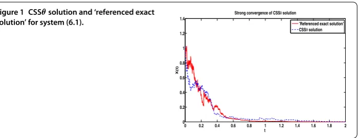
To show the convergence of the CSSθ method for system (.), we fixt= –,T= , λ= ,θ = .. Noting that the exact solution of nonlinear jump-diffusion system (.) is not available, we use the numerical solution by the SSBE method with step sizet= – as the ‘referenced exact solution’ (Theorem in [] can guarantee its strong convergence) in Figure .
In Figure , we show the numerical solution by the CSSθmethod with step sizet= – and the ‘referenced exact solution’. we can easy to find that the CSSθapproximation and the ‘referenced exact solution’ make no major difference between both paths. That is to say the CSSθmethod converges to the ‘referenced exact solution’ well. Hence our method is efficient for the nonlinear jump-diffusion systems.
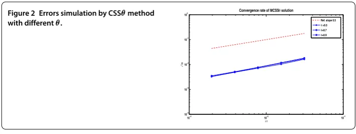
To show the strong convergence order of the CSSθmethod with different parameterθ, we fixT= ,λ= and changeθ= ., ., ., respectively. The ‘referenced exact solution’ of system (.) is also used by the SSBE method with step sizet= –. We simulate the numerical solutions with five different step sizesh= p–tfor ≤p≤,t= –. The mean-square errorsε= /,",i= |Yn(ωi) –X(T)|, all measured at timeT= , are
estimated by trajectory averaging. We plot our approximation to√againstton a log-log scale. For reference a dashed line of slope one-half is added.
In Figure , we see that the slopes of the four curves appear to match well. Therefore, the results verify the strong convergence order of the proposed method.
Figure 2 Errors simulation by CSSθmethod with differentθ.
Acknowledgements
This research is partial supported with funds provided by the National Natural Science Foundation of China (Grant Nos. 11501410, 11471243 and 11672207), and in part by Natural Science Foundation of Tianjin (No: 17JCQNJC03800). We thank the anonymous reviewers for their very valuable comments and helpful suggestions which improve this paper significantly.
Competing interests
The authors declare that they have no competing interests.
Authors’ contributions
All the authors contributed equally to this work. They all read and approved the final version of the manuscript.
Author details
1Department of Mathematics, Tianjin Polytechnic University, Tianjin, 300387, P.R. China.2Department of Sport Culture
and Communication, Tianjin University of Sport, Tianjin, 300381, P.R. China.
Publisher’s Note
Springer Nature remains neutral with regard to jurisdictional claims in published maps and institutional affiliations.
Received: 15 August 2016 Accepted: 16 June 2017 References
1. Bruti-Liberati, N, Platen, E: Strong approximations of stochastic differential equations with jumps. J. Comput. Appl. Math.205, 982-1001 (2007)
2. Chalmers, GD, Higham, DJ: Convergence and stability analysis for implicit simulations of stochastic differential equations with random jump magnitudes. Discrete Contin. Dyn. Syst., Ser. B9, 47-64 (2008)
3. Higham, DJ, Kloeden, PE: Convergence and stability of implicit methods for jump-diffusion. Int. J. Numer. Anal. Model. 3, 125-140 (2006)
4. Hu, L, Gan, SQ: Convergence and stability of the balanced methods for stochastic differential equations with jumps. Int. J. Comput. Math.88, 2089-2108 (2011)
5. Tan, JG, Mu, ZM, Guo, YF: Convergence and stability of the compensated split-stepθ-method for stochastic differential equations with jumps. Adv. Differ. Equ.2014, 209 (2014)
6. Wang, XJ, Gan, SQ: Compensated stochastic theta methods for stochastic differential equations with jumps. Appl. Numer. Math.60, 87-887 (2010)
7. Jiang, F, Shen, Y, Wu, FK: Jump systems with the mean-revertingγ-process and convergence of the numerical approximation. Stoch. Dyn.12, 1150018 (2012)
8. Bao, J, Mao, XR, Yin, G: Competitive Lotka-Volterra population dynamics with jumps. Nonlinear Anal.74, 6601-6616 (2011)
9. Higham, DJ, Mao, XR, Stuart, AM: Strong convergence of Euler-type methods for nonlinear stochastic differential equations. SIAM J. Numer. Anal.40, 1041-1063 (2002)
10. Hutzenthaler, M, Jentzen, A, Kloeden, PE: Strong and weak divergence in finite time of Euler’s method for stochastic differential equations with non-globally Lipschitz continuous coefficients. Proc. R. Soc. Lond., Ser. A, Math. Phys. Eng. Sci.467, 1563-1576 (2010)
11. Mao, XR, Szpruch, L: Strong convergence and stability of implicit numerical methods for stochastic differential equations with non-globally Lipschitz continuous coefficients. J. Comput. Appl. Math.238, 14-28 (2013)
12. Mao, XR, Szpruch, L: Strong convergence rates for backward Euler-Maruyama method for non-linear dissipative-type stochastic differential equations with super-linear diffusion coefficients. Stochastics85, 144-171 (2013)
13. Huang, CM: Exponential mean square stability of numerical methods for systems of stochastic differential equations. J. Comput. Appl. Math.236, 4016-4026 (2012)
14. Zong, XF, Wu, FK, Huang, CM: Exponential mean square stability of the theta approximations for neutral stochastic differential delay equations. J. Comput. Appl. Math.286, 172-185 (2015)
15. Zong, XF, Wu, FK, Huang, CM: Theta schemes for SDDEs with non-globally Lipschitz continuous coefficients. J. Comput. Appl. Math.278, 258-277 (2015)
17. Higham, DJ, Kloeden, PE: Strong convergence rates for backward Euler on a class of nonlinear jump-diffusion problems. J. Comput. Appl. Math.205, 949-956 (2007)