R E S E A R C H
Open Access
Asymptotic behavior of a diffusive
eco-epidemiological model with an infected
prey population
Wonlyul Ko
1, Wonhyung Choi
1and Inkyung Ahn
2**Correspondence: [email protected] 2Department of Mathematics, Korea
University, Sejong-ro Sejong, 30019, South Korea
Full list of author information is available at the end of the article
Abstract
We study a diffusive predator-prey system with a ratio-dependent functional response when a prey population is infected under homogeneous Neumann boundary condition. All non-negative and positive equilibria are investigated, and the conditions that give rise to asymptotic behavior of these equilibria are examined. In particular, we present a biological interpretation of disease-free and total extinction states. A comparison principle and the stability analysis for the parabolic problem are employed.
MSC: 35B35; 35K57; 92D25
Keywords: predator-prey model; ratio-dependent functional response; locally/globally asymptotical stability; disease free
1 Introduction
We focus on the diffusive predator-prey system with a ratio-dependent functional re-sponse and disease in the prey; specifically,
⎧ ⎪ ⎪ ⎪ ⎪ ⎪ ⎪ ⎪ ⎪ ⎨ ⎪ ⎪ ⎪ ⎪ ⎪ ⎪ ⎪ ⎪ ⎩
ut–du=u[r–Kru–mwα+wu+v–bv],
vt–dv=v[bu–d–mwβ+wu+v],
wt–Dw=w[–d+mwc+αuu+v+mwc+βvu+v] in (,∞)×, ∂u
∂η= ∂v
∂η= ∂w
∂η = on (,∞)×∂,
u(,x) =u(x), v(,x) =v(x), w(,x) =w(x) in,
(.)
where⊆RN is a bounded region with smooth boundary∂, andr,m,K,b,di,Di,c, α, andβare positive constants;a,b,b,landkare positive constants as well. The initial
functionsu,v, andware not identically zero in ;u,v, andwrepresent the
densi-ties of the susceptible prey, infected prey, and predator, respectively, andηis the outward directional derivative normal to∂. Furthermore,α andβ are the searching efficiency constants of the predation rate for the susceptible and infective prey, respectively.mα and
β
m are the maximum per capita capturing rates of the predator for the susceptible prey and infected prey, respectively.mis the predation rate for the susceptible prey and in-fected prey. Finally,bis the force of infection,danddare the death rates of the infected
prey and predator, respectively, andcis a conversion rate. The homogeneous Neumann boundary condition describes an environment with no flux at the boundary of the region. During the last three decades, various types of predator-prey models are studied exten-sively by many researchers. Many models have a functional response in which ignoring an effect of predator density,i.e., the function that describe a density of prey which is consumed by its predator depends only on prey. However, there is explicit biological and physiological evidence [–] that in many situations, when predator have to search for food, a more suitable general predator-prey model in heterogeneous situations should be had the ratio-dependent functional response, which the per capita predator growth rate should be a function of the ratio of prey to predator abundance. Ratio-dependent mod-els have been mathematically studied for both the spatially homogeneous case [–] and the spatially inhomogeneous case [–]. In [, ], one examined the model of Arditi and Ginzburg []. One showed that under some conditions, the whole population can be extinct.
On the other hand, epidemic models have also received a lot of attention since Kermack-McKendrick’s model. Among them, we are interested in eco-epidemiological systems with predator-prey interactions. Considerable research has been done on the spatially homo-geneous case [–].
In the real application, diffusive system in this study can be used to describe the in-teraction between marine viruses in aquatic ecosystems and the species [, ], since there is evidence that viral infection might accelerate the termination of phytoplankton blooms []. In fact, in [], the authors showed experimentally that viral disease can infect bacteria and phytoplankton in coastal water. In [, , ], they observed oscilla-tions and waves in a phytoplankton-zooplankton system with Holling-type II and III graz-ing under lysogenic viral infection and frequency-dependent transmission. Hilker [] also investigated the local dynamics of phytoplankton with lytic infection and frequency-dependent transmission as well as zooplankton with Holling-type II grazing.
Arinoet al.[] suggested the non-dimensionalized model, which is a non-spatial ver-sion of (.). There, the authors obtained the conditions for which no trajectory can reach the origin following any fixed direction or spirally. Also the criteria of persistence were found. The above studies have been done mostly for the non-spatial case.
In this paper, we investigate the conditions of the asymptotic behavior of a unique pos-itive constant solution and the non-negative equilibria of (.), which is a spatially depen-dent model with diffusion.
Model (.) is based on the following assumptions:
(a) In the absence of disease, the prey population grows according to logistic law with carrying capacityK> and an intrinsic growth rater> .
(b) In the presence of disease, the prey consists of two classes: susceptible prey and infected prey.
(c) Only susceptible prey can reproduce themselves logistically and contribute to its carrying capacity. Infected prey do not grow, recover, or reproduce.
(d) Disease can only be spread among the prey, and it is not inherited. Disease transmission follows the simple law of mass action.
The model of Hamiltonet al.[] showed that infected individuals do not contribute in the reproduction process; infection reduces the remaining capacity due to the inability to compete for resources. Thus, we may assume that the growth term of the susceptible population follows only the law of logistic growth.
For additional background information pertaining to (.), we refer to [] and the ref-erences therein.
The remainder of this paper is organized as follows. In Section , we investigate the large time behavior of non-negative constant solutions and the asymptotic stability of a positive constant solution. Finally, the results obtained are analyzed in terms of biological interpretations in Section .
2 Asymptotical behavior of constant solutions
In this section, the asymptotic behavior of non-negative and positive constant solutions to (.) is examined.
For convenience, we denote the growth rate terms as follows:
f(u,v,w) :=r– r Ku–
αw
mw+u+v–bv,
f(u,v,w) :=bu–d–
βw mw+u+v,
f(u,v,w) := –d+ cαu mw+u+v+
cβv mw+u+v.
Using the uniform bound ofu, vandw, one can show that (uf,vf,wf) satisfies the
Lipschitz condition. Using the upper and lower solution method in [], it can also be shown that (.) has a non-negative solution.
The next theorem states that the solution to (.) is uniformly bounded [].
Theorem . The solution(u,v,w)of(.)is uniformly bounded;specifically,
≤u(t,x)≤B, ≤v(t,x)≤B, ≤w(t,x)≤B,
where Biis defined by
B:=max
K,u∞
,
B:=max
d K
r r+d
,u∞+v∞
,
B:=max
w∞,c(α+β) –d dm
B
.
The dissipation and persistence of the parabolic system (.) can be found in [].
Theorem . For a solutionu= (u(t,x),v(t,x),w(t,x))to the parabolic system(.),
lim sup
t→∞ u≤ K,
d K
r r+d
,c(α+β) –d
dm
d K
r r+d
Theorem . Assume thatβ≥α>d
System (.) has the following non-negative equilibria:
⎧
Furthermore, if the following conditions are satisfied:
AS+BS+C< and d<cβ, (.)
2.2 Asymptotic stability of equilibria
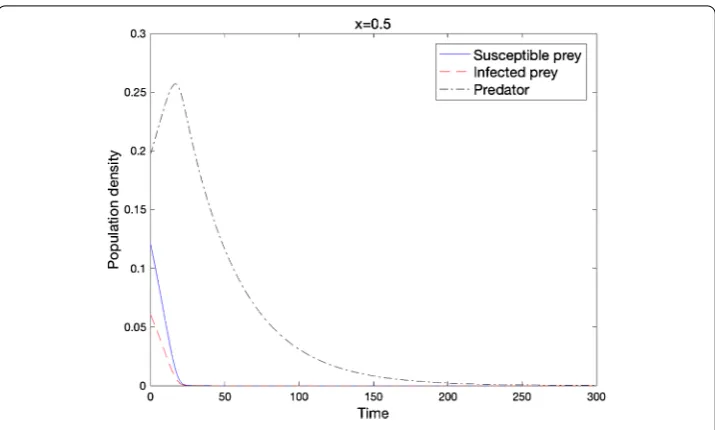
Figure 1 Local stability of e0when the condition of Theorem 2.4 holds
(d= 0.01,D= 0.01,r= 0.05,b= 0.430,d1= 0.03,d2= 0.6,K= 1.0,α= 1.2,β=α,c= 1.0,m= 0.08).
.. Asymptotic stability ofe
We investigate the stability at (, , ). For the stability of e, we assumed=D.
Figure shows that under some conditions, all three species become extinct. We point out that the corresponding non-spatial model had the same asymptotic behavior under the same condition in the following theorem.
Theorem . Assume that mc≤,β≥α,min{cα–d,+αm} ≥r.If the initial data satisfies w≥u+v,thenlimt→∞u= e.
Proof Subtracting the first and second equations from the third equation in (.) yields
(w–u–v)t–d(w–u–v) =wf–uf–vf
= (w–u–v)f+ (f–f)v+ (f–f)u. (.)
Also note that
f–f=
cαu+cβv+βw
mw+u+v –d–bu+d
=cαu+
β αv+
β
cαw
mw+u+v –d–bu+d
≥cα–d+d–bu,
f–f=
cαu+cβv+αw
mw+u+v –d–r+ r Ku+bv
=cαu+
β αv+
cw
mw+u+v –d–r+ r Ku+bv
hold under the assumptions thatmc≤ andβ≥α. As a result, (f–f)v+ (f–f)u≥
(cα–d+d)v+ (cα–d–r+Kru)u≥, sincecα–d≥r. Thus, applying the positivity
lemma [] to (.),w≥u+vholds ifw≥u+v. In the light of these facts, the main
result is satisfied; specifically,
ut–du=u
r– r
Ku–
αw
mw+u+v–bv
≤u
r– r
Ku–
αw mw+w
=u
r– r
Ku–
α
m+
≤,
since+αm≥r. Thus,limt→∞w= on. Consequently,limt→∞u= andlimt→∞v= on
sincew≥u+v.
Theorem .
(i) If there exists a positive constantθsuch that rm–α+dm≤(cα–r–d)θ,
dm–dm–β≤(cβ+d–d)θ,
(.)
holds,then the region={(u,v,w) :u,v,w≥,u+v≤θw}is an invariant set for
(.).
(ii) In addition to(.),if–m+α
r ≥θ,limt→∞u=efor the initial function (u,v,w)∈.
(iii) In addition to(.),ifcmax{α,β} ≤d,limt→∞u=efor the initial function
(u,v,w)∈.
(iv) In addition to(.),ifcβ≥cα>dandθ<cdα–md,limt→∞u=efor the initial function(u,v,w)∈.
Proof (i) LetG(u,v,w) =u+v–θw. To achieve the desired result, Corollary . of [] is used; in particular, we will show that (uf,vf,wf) points intoon∂. On the boundary
of(except for the boundaryu+v=θw),dG·(uf,vf,wf)≤ can easily be verified.
It is straightforward to show thatdG·(uf,vf,wf)≤ on the boundaryu+v=θw. In
fact,
dG·(uf,vf,wf)
= (, , –θ)·(uf,vf,wf)
=uf+vf–θwf
=u
r– r
Ku–
αw mw+θw–bv
+v
bu–d–
βw mw+θw
–θw
–d+
cαu mw+θw+
cβv mw+θw
=u r– α
The last inequality holds by assumption (.).
(ii) Since is an invariant region under assumption (.), u +v≤θw holds for
Consider the third equation in (.):
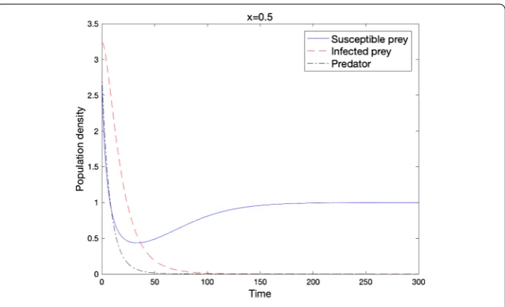
Figure 2 Local stability of e1when the condition of Theorem 2.6 holds
(d= 0.01,D= 0.01,r= 0.5,b= 0.430,d1= 1.0,d2= 2.0,K= 1.0,α= 1.2,β=α,c= 1.0,m= 10.0).
Letτ=[ +θcβ–d
dm ]. Under the assumption thatθ<
dm
cα–d,τ< is satisfied. Sinceρ() =
θcβ–d
dm ρ<τρ, if a sufficiently smallε> is chosen such thatρ(ε) <τρ,u(t,x) +v(t,x)≤
θ[cβ–d
dm (ρ+ε) +ε] <τρonfort≥T.
Now, consider (.) under the restriction thatu(t,x) +v(t,x)≤τρ. Thenlim supt→∞w
≤cβ–d
dm τρ. Thus, there exists aT≥Tsuch thatw(t,x)≤
cβ–d
dm τρ+εonfor timet≥T.
Again,u(t,x) +v(t,x)≤θ[cβ–d
dm (τρ) +ε]≤τ
ρonfort≥T
and for a sufficiently small
ε> .
Inductively, there exists a sequenceTnwithTn→ ∞such thatu(t,x) +v(t,x)≤τnρon fort≥Tn. Moreover, sinceτ< ,u+v→ uniformly onast→ ∞. Consequently,w goes to zero ast→ ∞as well.
.. Asymptotic stability ofe
In this subsection, we investigate the stability at (K, , ) under the following conditions:
d≥bK, d≥cα and r>
α
m. (.)
The next result implies that only the susceptible prey can survives (Figure ).
Theorem . Under assumption(.),limt→∞u= euniformly on.
Proof From Theorem ., we already knowlim supt→∞u≤K. Furthermore, sinced≥ bK,vt–dv=vf(u,v,w)≤ impliesv→ uniformly onast→ ∞. Thus there exists
aT> such thatv≤εfor an arbitraryε> andt≥T. Sinceεis arbitrary, the
assump-tion thatd≥cαand the comparison principle implyw→ uniformly onast→ ∞.
Therefore, there existsT≥Tsuch thatw≤εfort≥T.
Note thatlim inft→∞u≥(r–bε– α
m) K
r :=can also be obtained using the methods from Theorem .. Sinceuf(u,v,w)≥u[r–Kru– mαεε+u–bε]≥u[r–
r Ku–
αε
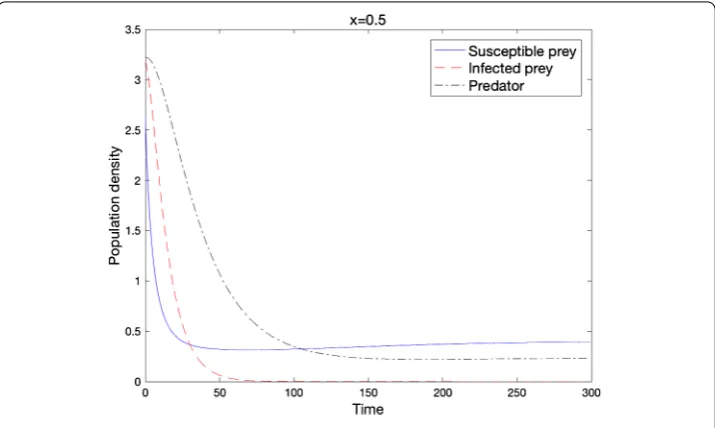
Figure 3 Local stability of e2when the condition of Theorem 2.7 holds
(d= 0.01,D= 0.01,r= 0.5,b= 0.430,d1= 1.0,d2= 0.5,K= 1.0,α= 3.5,β=α,c= 1.0,m= 10.0).
fort≥T,lim inft→∞u≥(r–bε–(m–)αεε+)
K
r >follows from the comparison principle. Therefore, sinceεis arbitrary,limt→∞u=euniformly on.
.. Asymptotic stability ofe
We investigate the stability at (K( –cα–d
cmr ), , cα–d
dm K( –
cα–d
cmr )) under the following con-dition:
rmd≤(rm–α)(cα–d), bK<d and <cα–d<cmr. (.)
For simplicity, letu∗=K( –cα–d
cmr ) andw∗=
cα–d
dm u ∗ .
The following theorem indicates that one can control the infected prey, namely, only the infected prey can be removed out under some conditions (Figure ).
Theorem . Under assumption(.),limt→∞u= euniformly on.
Proof We prove this theorem by induction. First, consider the following parabolic prob-lem:
⎧ ⎪ ⎪ ⎨ ⎪ ⎪ ⎩
ut–du=u(r–Kru) in (,∞)×, ∂u
∂η = on (,∞)×∂, u(,x) =u(x) in.
Then there exists aT> such thatu≤u∗(≡K) +εonfort≥Tand a sufficiently smallsuch thatd
Next, consider the following problem under the condition thatbK<d:
Consider the following problem:
⎧ Consider the following problem:
⎧
Consider the following problem:
⎧
For induction, consider the following problems forTn–≤Tn–
⎧
bounded from above, the limits of these sequences exist. Denote these limits byu,w,u, andw, respectively. Consequently,u≤u∗≤uandw≤w∗≤w. The following also holds:
⎧ ⎪ ⎪ ⎪ ⎪ ⎪ ⎨ ⎪ ⎪ ⎪ ⎪ ⎪ ⎩
u=Kr(r–mwαw+u),
w=cα–d
dm u,
u=Kr(r–mwαw+u),
w=cα–d
dm u.
(.)
Suppose to the contrary thatu=u. The first and third equations in (.) can be rewritten as
r– r
Ku–
αcα–d
dm u mcα–d
dm u+u
= ,
r– r
Ku–
αcα–d
dm u mcα–d
dm u+u
= ,
respectively. These two equations imply
⎧ ⎨ ⎩
(rm–α)cα–d
dm u+ru–
r Km
cα–d
dm uu–
r
Kuu = , (rm–α)cα–d
dm u+ru–
r Km
cα–d
dm uu–
r
Kuu = .
(.)
Subtracting the second equation from the first equation in (.) yields
(u–u) r– r
K(u+u) – (rm–α) cα–d
dm
= .
By assumption, sinceu=u(i.e.,u>u),A:=r– r
K(u+u) – (rm–α) cα–d
dm must be zero. But
A<r– (rm–α)cα–d
dm ≤ from (.). Hence,u=u=u ∗
; likewise,w=w=w∗. Consequently,
as timetgoes to infinity (i.e.,n→ ∞),
u∗–ε≤u≤u∗+ε,
≤v≤ε,
w∗–ε≤w≤w∗+ε,
are satisfied for an arbitraryε> . Therefore, the desired result is achieved.
In the following theorem, we modify the condition thatbK<din (.) by reversing the
inequality,i.e.,bK>d, sincebK<dcausesvto converge to zero automatically.
Theorem . If the following conditions hold:
rmd≤(rm–α)(cα–d),
d<bK<d+
βσ
<cα–d<cmr,
r> α
m+bθ,
whereθ:=
d
K r(
r+d )
andσ:=cα–d
dm (r– α
m–bθ) K
r,thenlimt→∞u= euniformly on.
Proof First, note that there exists aT> such thatu≤K+εandu+v≤θ+εfort≥T
andx∈, as in Theorem ..
Consider the following parabolic problem:
⎧ ⎪ ⎪ ⎨ ⎪ ⎪ ⎩
Ut–dU=U(r–mα –b(θ+ε) –KrU) in (T,∞)×, ∂U
∂η = on (T,∞)×∂, U(,x) =u(T,x) in.
Then there existsT≥Tsuch thatu≥(r–mα –bθ)Kr –εonfort≥T. It follows that w≥σ–εfort≥Tandx∈whereT≥T. Now, we are ready to prove thatlimt→∞v=
uniformly on.
Consider the following problem:
⎧ ⎪ ⎪ ⎨ ⎪ ⎪ ⎩
Vt–dV=V(b(K+ε) –m(σβ(–σε–)+εθ)+ε–d) in (T,∞)×, ∂V
∂η = on (T,∞)×∂, V(,x) =v(T,x) in.
(.)
For a sufficiently smallε> , the right hand side of the first equation in (.) is negative becausebK<d+mβσσ+θ.
Hence, similar to Theorem ., there existsT≥Tsuch that ≤v≤εfort≥T. The
remainder of this proof follows using the same argument as Theorem ..
.. Asymptotic stability ofe
In this subsection, we investigate the stability at (d
b,
b(r– r K
d
b), ). Before developing our argument, we define the following notation, which is similar to the notation defined in [, ].
Notation .
(i) μi: Eigenvalue of–onunder Neumann boundary condition.
(ii) E(μi): The eigenspace corresponding toμi.
(iii) {ϕij:j= , . . . ,dimE(μi)}: An orthonormal basis ofE(μi). (iv) Xij={c·ϕij|c∈R}.
(v) X={u= (u,v,w)∈[C()]|∂u
∂η= ∂v
∂η= ∂w
∂η = on∂}.
The eigenvalues in (i) satisfy =μ<μ<μ<· · · → ∞. Also, X =
∞
i=Xi, where Xi= dimE(μi)
j= Xij. Now, we show the local stability at e.
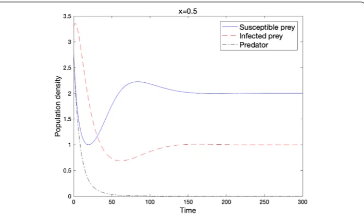
The susceptible prey and the infected prey may survive together without the predator (Figure ).
Theorem . Ifmax{α,β}<d
c and d(r+bK) >bK>d
,then equilibriumeof(.)
Figure 4 Local stability of e3when the condition of Theorem 2.10 holds
(d= 0.01,D= 0.01,r= 1.5,b= 0.5,d1= 1.0,d2= 2.0,K= 3.0,α= 1.5,β=α,c= 1.0,m= 10.0).
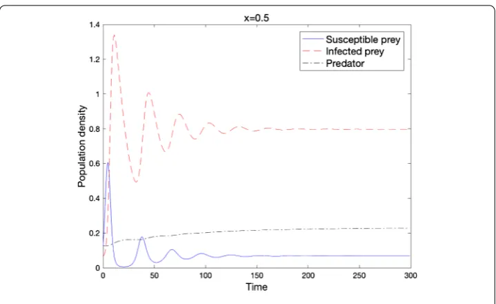
Figure 5 Local stability of u∗when the condition of Theorem 2.11 holds
(d= 0.01,D= 0.01,r= 0.3699,b= 0.430,d1= 0.0291,d2= 0.0069,K= 0.9299,α= 0.0122,β=α, c= 8.0999,m= 50.3).
τi=bu∗v∗d+ r
Ku ∗ d+
r Ku
∗
D
+ r
Ku ∗
+
r K +
d+
r K
u∗u∗–bu∗v∗
D> ,
τi= r
Kb u∗
v∗+ r Ku
∗ +
r K
u∗u∗–bu∗v∗
> .
Hence,AiBi–Ci> for alli≥. From the Routh-Hurwitz criterion for eachi, the three roots ofλ+Aiλ+Biλ+Ci= have negative real parts sinceAi,Ci, andAiBi–Ci> . The remainder of this proof follows from Theorem .. in [].
.. Asymptotic stability ofu∗
We investigate the asymptotic stability of the positive equilibrium point under (.) and the following conditions:
⎧ ⎪ ⎪ ⎨ ⎪ ⎪ ⎩
mc≥, α=β,
d<cα,
max{db
cα,α
cα–d
dm
b d} ≤
r K≤
bd α
dm
cα–d.
(.)
Here, we can choose numerical values that satisfy condition (.) and (.), for example,
r= .,b= .,d= .,K= .,α=β= .,m= .,c= ., and d= ..
The final result says that all three species can survives together under specific conditions (Figure ).
Proof The linearization of (.) is ut= (D+ Fu(u∗))u at the constant solution u∗, where
The following notation is adopted for simplicity:
Fu(u∗) =
Sincew∗=cαd–md(u∗+v∗),b(u∗+v∗) =r–
r
Ku∗+dandr– r Ku∗> ,
LL+LL+LL–LL–LL–LL
=bu∗v∗+ r
Kα
u∗w∗
(mw∗+u∗+v∗)
mcw∗+ (mc– )v∗> ,
LL+LL–LL–LL= r Kmcu∗α
(u∗+v∗)w∗
(mw∗+u∗+v∗) > ,
LL–LL
=u∗v∗ –α r K
w∗
(mw∗+u∗+v∗) +b
=u∗v∗ –α r K
cα–d dm
u∗+v∗
(mw∗+u∗+v∗) +b
≥u∗v∗ –αr
K cα–d
dm
u∗+v∗ +b
=u∗v∗ –α r K
cα–d dm
b r–Kru∗+d
+b
>u∗v∗b –α r
K cα–d
dm
d
+b
>
and
–LLL–LLL–LLL+LLL+LLL+LLL
=cαbmu∗v∗w∗ u∗+v∗
(mw∗+u∗+v∗) > .
It follows thatAiBi–Ci=τiμi +τiμi+τiμi+τi, where
τi= d(d+D)D+d,
τi=d(–L– L– L) +D(–L–L) + dD(–L–L–L) > ,
τi=d(LL+LL+LL–LL–LL–LL) + (LL–LL)
+d(–L–L–L)(–L–L– L) +D(–L–L–L)(–L–L)
+D(–L–L)(–L) + (–LL) + (–LL)
> ,
τi= –LLL–LLL+LLL+LLL–LLL–LLL
–LLL+LLL+LLL–LLL–LLL+LLL
+LLL–LLL+LLL+LLL.
The positivity ofτiandτifollows directly from the above calculations. Now, we investi-gate the sign ofτiforLL=LL. Note that
–L=u∗ r K –
αw∗
(mw∗+u∗+v∗)
=u∗ r K –α
cα–d dm
u∗+v∗
(mw∗+u∗+v∗)
>u∗ r K –α
cα–d dm
u∗+v∗
=u∗ r K –α
cα–d dm
b r–Kru∗+d
>u∗ r K –α
cα–d dm
b d
≥,
sincew∗=cα–d
dm (u∗+v∗),b(u∗+v∗) =r–
r
Ku∗+d, andr– r
Ku∗> . Finally, sinceL=L, we obtain the positivity of
τi= (–L–L)(LL–LL) + (–L)(–L)(–L–L)
+ (–L)L(–L–L) +ϒ> ,
where
ϒ=LLL+LLL+LLL+LLL
=L (mc– )α(u∗+v∗) u∗v∗w∗
(mw∗+u∗+v∗)+ (mc– )α (u
∗+v∗) u ∗w∗
(mw∗+u∗+v∗)
+ α(u∗+v∗)
(mw∗+u∗+v∗)(–L)
> .
Hence,AiBi–Ci> for alli≥. From the Routh-Hurwitz criterion for eachi, the three roots ofλ+Aiλ+Biλ+Ci= have negative real parts sinceAi,Ci, andAiBi–Ci> . The remainder of this proof follows from Theorem .. in [].
3 Conclusion
A diffusive predator-prey model with a ratio-dependent functional response and infected prey population was investigated under homogeneous Neumann boundary conditions. We showed that depending on initial data, all species can become extinct if the predation rate is small and the searching efficiency constant of the predation rate of the predator for the susceptible prey is large; in other words, the predator overeats the susceptible prey. On the other hand, we showed that the infected prey becomes extinct if the death rate of the infected prey is sufficiently large without respect to the initial data. Furthermore, the same conclusion holds even if the death rate of the infected prey is relatively small. In [], the authors proposed a model by considering that the encounter infection rate is meaningful only in the case that it follows the law of ratio-dependence and not the law of simple mass action. They showed that the model exhibits parasite-induced host extinction. Such an ex-tinction is similar to that induced by a ratio-dependent predator-prey functional response. The stability of the disease-free equilibrium eimplies that under certain conditions, total extinction is not possible and the introduction of infected prey into the system may act as a biological control to save the ecosystem from extinction.
As regards application, the model with ratio-dependent functional response in this study can be used and improved to describe the interaction among the diseased-species in ecosystems, the susceptible species, and additional species with a certain biological prop-erty.
Acknowledgements
This work was supported by a Korea University Grant.
Competing interests
The authors declare that they have no competing interests.
Authors’ contributions
All authors equally made contributions and approved the final version of this manuscript.
Author details
1Department of Mathematics, Korea University, Anam-dong Seoul, 02841, South Korea.2Department of Mathematics,
Korea University, Sejong-ro Sejong, 30019, South Korea.
Publisher’s Note
Springer Nature remains neutral with regard to jurisdictional claims in published maps and institutional affiliations.
Received: 28 March 2017 Accepted: 20 July 2017
References
1. Arditi, R, Ginzburg, L, Akcakaya, H: Variation in plankton densities among lakes: a case for ratio-dependent models. Am. Nat.138, 1287-1296 (1991)
2. Arditi, R, Saiah, H: Empirical evidence of the role of heterogeneity in ratio-dependent consumption. Ecology73, 1544-1551 (1992)
3. Cosner, C, DeAngelis, D, Ault, J, Olson, D: Effects of spatial grouping on the functional response of predators. Theor. Popul. Biol.56, 65-75 (1999)
4. Gutierrez, A: The physiological basis of ratio-dependent predator-prey theory: a metabolic pool model of Nicholson’s blowflies as an example. Ecology73, 1552-1563 (1992)
5. Hsu, S, Hwang, T, Kuang, Y: Global analysis of the Michaelis-Menten-type ratio-dependent predator-prey system. J. Math. Biol.42(6), 489-506 (2001)
6. Hsu, S, Hwang, T, Kuang, Y: Rich dynamics of a ratio-dependent one-prey two-predators model. J. Math. Biol.43(5), 377-396 (2001)
7. Hsu, S, Hwang, T, Kuang, Y: A ratio-dependent food chain model and its applications to biological control. Math. Biosci.181(1), 55-83 (2003)
8. Kuang, Y, Beretta, E: Global qualitative analysis of a ratio-dependent predator-prey system. J. Math. Biol.36, 389-406 (1998)
9. Cantrell, R, Cosner, C: On the dynamics of predator-prey models with the Beddington-DeAngelis functional response. J. Math. Anal. Appl.257(1), 206-222 (2001)
10. Pang, P, Wang, M: Qualitative analysis of a ratio-dependent predator-prey system with diffusion. Proc. R. Soc. Edinb. A 133(4), 919-942 (2003)
11. Ryu, K, Ahn, I: Positive solutions to ratio-dependent predator-prey interacting systems. J. Differ. Equ.218, 117-135 (2005)
12. Jost, C, Arino, O, Arditi, R: About deterministic extinction in ratio-dependent predator-prey models. Bull. Math. Biol. 61, 19-32 (1999)
13. Arditi, R, Ginzburg, L: Coupling in predator-prey dynamics: ratio dependence. J. Theor. Biol.139, 311-326 (1989) 14. Beltrami, E, Carroll, T: Modelling the role of viral disease in recurrent phytoplankton blooms. J. Math. Biol.32, 857-863
(1995)
15. Chattopadhyay, J, Arino, O: A predator-prey model with disease in the prey. Nonlinear Anal.36, 747-766 (1999) 16. Chattopadhyay, J, Pal, S: Viral infection of phytoplankton-zooplankton system- a mathematical modeling. Ecol. Model.
151, 15-28 (2002)
17. Hadeler, K, Freedman, H: Predator-prey population with parasite infection. J. Math. Biol.27, 609-631 (1989) 18. Venturino, E: Epidemics in predator-prey models: disease in the prey. In: Arino, O, Axelrod, D, Kimmel, M, Langlais, M
(eds.) Mathematical Population Dynamics: Analysis of Heterogeneity, vol. 1, pp. 381-393 (1995)
19. Xiao, Y, Chen, L: A ratio-dependent predator-prey model with disease in the prey. Appl. Math. Comput.131, 397-414 (2002)
20. Xiao, Y, Chen, L: Analysis of a three species eco-epidemiological model. J. Math. Anal. Appl.258, 733-754 (2001) 21. Fuhrman, JA: Marine viruses and their biogeochemical and ecological effects. Nature399, 541-548 (1999) 22. Gastrich, MD, Leigh-Bell, JA, Gobler, CJ, Anderson, OR, Wilhelm, SW, Bryan, M: Viruses as potential regulators of
regional brown tide blooms caused by the alga. Aureococcus anophagefferens. Estuaries27(1), 112-119 (2004) 23. Jacquet, S, Heldal, M, Iglesias-Rodriguez, D, Larsen, A, Wilson, W, Bratbak, G: Flow cytometric analysis of an Emiliana
huxleyi bloom terminated by viral infection. Aquat. Microb. Ecol.27, 111-124 (2002)
25. Malchow, H, Hilker, F, Petrovskii, SV, Brauer, K: Oscillations and waves in a virally infected plankton system. Part I: the lysogenic stage. Ecol. Complex.1(3), 211-223 (2004)
26. Malchow, H, Hilker, F, Sarkar, R, Brauer, K: Spatiotemporal patterns in an excitable plankton system with lysogenic viral infection. Math. Comput. Model.42(9-10), 1035-1048 (2005)
27. Hilker, F, Malchow, H: Strange periodic attractors in a prey-predator system with infected prey. Math. Popul. Stud.13, 119-134 (2006)
28. Arino, O, Abdllaoui, A, Mikram, J, Chattopadhyay, J: Infection in prey population may act as a biological control in raito-dependent predator-prey models. Nonlinearity17, 1101-1116 (2004)
29. Uhlig, G, Sahling, G: Long-term studies on Noctiluca scintillans in the German bight Neth. J. Sea Res.25, 101-112 (1992)
30. Hamilton, WD, Axelrod, R, Tanese, R: Sexual reproduction as an adaptation to resist parasite. Proc. Natl. Acad. Sci. USA 87, 3566-3573 (1990)
31. Pao, C: Nonlinear Parabolic and Elliptic Equations. Plenum, New York (1992)
32. Ko, W, Ahn, I: Pattern formation of a diffusive eco-epidemiological model with predator-prey interaction. Preprint 33. Smoller, J: Shock Waves and Reaction-Diffusion Equations. Springer, New York (1983)
34. Lin, Z, Pedersen, M: Stability in a diffusive food-chain model with Michaelis-Menten functional response. Nonlinear Anal.57, 421-433 (2004)
35. Pang, P, Wang, M: Strategy and stationary pattern in a three-species predator-prey model. J. Differ. Equ.200, 245-273 (2004)
36. Henry, D: Geometric Theory of Semilinear Parabolic Equations. Lecture Notes in Mathematics, vol. 840. Springer, Berlin (1993)