R E S E A R C H
Open Access
Nonstandard finite difference variational
integrators for nonlinear Schrödinger
equation with variable coefficients
Cuicui Liao and Xiaohua Ding
**Correspondence:
Department of Mathematics, Harbin Institute of Technology at Weihai, 2 Wenhua West Road, Weihai, Shandong 264209, China
Abstract
In this paper, the idea of nonstandard finite difference discretization is employed to develop two variational integrators for the nonlinear Schrödinger equation with variable coefficients. These integrators are naturally multi-symplectic, and their multi-symplectic structures are presented by the multi-symplectic form formulas. Local truncation errors and convergences of the integrators are briefly discussed. The effectiveness and efficiency of the proposed schemes, such as the convergence order, numerical stability, and the capability in preserving the norm conservation, are verified in the numerical experiments.
Keywords: variational integrators; nonstandard finite difference; multi-symplectic; Schrödinger equation
1 Introduction
The nonlinear Schrödinger equation (NLSE) [, ]
iut+uxx+V
|u|u= ,
has wide applications in many areas such as quantum mechanics, nonlinear optics, and
plasma physics,etc.Extensive efforts have been devoted to studying the equation
theo-retically and numerically due to its broad and important applications. Various numerical methods for the nonlinear Schrödinger equation [–] such as finite element methods [],
finite difference methods [], spectral method [],etc.have been developed. Among these
numerical methods of different categories, the multi-symplectic method has attracted special attention for its better numerical stability for long-time computations and perfect performance in preserving the multi-symplecticity of NLS equations, which is an intrinsic conservative property of the Schrödinger equations.
In this paper, we consider the nonlinear Schrödinger equation with variable coefficients
iut+α(t)uxx+β(t)|u|u= , ()
wherei=√–,α(t) andβ(t) are integrable real functions int, andu(x,t) is a scalar field function with two independent variables labeled byxandt.
The nonlinear Schrödinger equation () can be reformulated as a multi-symplectic
Hamiltonian system []. Honget al.[, ] proposed a numerical scheme for the NLSE
with variable coefficients () by means of Preissman integrator []. For this Preissman in-tegrator, they derived a discrete multi-symplectic structure, named multi-symplectic con-servation law []. Also, the discrete normal concon-servation law and a global energy transit formula in temporal direction were shown in their paper.
It is a classical way to derive multi-symplectic numerical schemes from the Hamiltonian point of view [, , ]. After applying a numerical discretization to Hamilton’s equation [–], however, we need to rederive the discrete multi-symplectic conservation law since it is unclear what is geometrically conserved by this discretization. On this aspect, another classical way,i.e., deriving the multi-symplectic numerical schemes from the Lagrangian viewpoint and variational principle, has more advantages since it leads in a natural way to multi-symplectic integrators, and the discrete multi-symplectic structures are obtained
at the same time. Based on this Lagrangian viewpoint, Chenet al.[–] have
elabo-rately studied the variational multi-symplectic integrators for the nonlinear Schrödinger equation. By the discrete variational principle with the discrete Lagrangian function, the discrete variational integrator is derived, and the corresponding multi-symplectic struc-ture,i.e., the multi-symplectic form formula by Marsden [, ], is also obtained from the variational principle. In this work, we follow this Lagrangian viewpoint to study the multi-symplectic methods for the nonlinear Schrödinger equation with variable coefficients (). In this process, the discrete Lagrangian function needs to be defined for the discrete variational principle. The Lagrangian function can be discretized by using finite difference methods. In our paper, we use the nonstandard finite difference methods rather than the classical finite difference methods to approximate the Lagrangian function. The nonstan-dard finite difference methods developed by Mickens [–] have better performances than the classical ones in terms of numerical stability, and they can be constructed flexibly to preserve some important properties and conservation laws of the original models. The rules of designing nonstandard finite difference schemes are listed in Section .
Combining the ideas of discrete variational integrators and the nonstandard finite dif-ference methods is our starting point to study the nonlinear Schrödinger equation with variable coefficients (), which can be reformulated as the following Euler-Lagrange equa-tion:
∂L ∂u=
d dt
∂L ∂ut
+ d
dx ∂L ∂ux
, ()
with the Lagrangian function
L(u,ut,ux) =
α(t)uxu¯x+
i(uu¯t–uu¯ t) –
β(t)(uu¯)
, ()
whereu¯andu¯xare the conjugates ofuandux, respectively.
section. Section is devoted to showing the numerical performances of the developed nonstandard finite difference variational integrators. It also shows that our methods have a good performance in preserving the norm conservation law.
2 Discrete variational integrators and nonstandard finite difference methods In this section, we first introduce the concepts of discrete variational integrators, the corre-sponding multisymplectic structures, and the rules of nonstandard finite difference meth-ods.
2.1 Discrete variational integrators and multi-symplectic form formulas
Assume that we have a regular quadrangular mesh in the base space, with mesh lengths
xandt. The nodes in this mesh are denoted by (j,k)∈Z×Z, corresponding to the points (xj,tk) := (jx,kt) inR. We denote the value of the fielduat the node (j,k) byukj.
When we consider the triangle discretization, we denote a triangle at (j,k) with ordered triple ((j,k), (j+ ,k), (j,k+ )) byjk. DefineXto be the set of all such triangles. Then the
discrete jet bundle [, ] is defined as follows:
JY:=ukj,ukj+,ukj+∈R:(j,k), (j+ ,k), (j,k+ )∈X,
which equalsX×R.
Let us posit a discrete LagrangianLd:JY→R. Given a trianglejk, define the function LdbyLd(ukj,ukj+,ukj+) which is a discrete version of the Lagrangian density []. Then the
action functional can be defined as
S=· · ·+Ld
uk
j,ukj+,ukj+
+Ld
uk
j–,ukj,ukj–+
+Ld
uk–
j ,ukj+–,ukj
+· · ·.
By the discrete variational principle [], we obtain the discrete Euler-Lagrange equation by keeping the values of the field on the boundary fixed and taking variations with respect toukj,
DLd
uk
j,ukj+,ukj+
+DLd
uk j–,ukj,uk
+
j–
+DLd
uk–
j ,uk
–
j+,ukj
= .
The discrete Euler-Lagrange equation is the so-called discrete variational integrator. Meanwhile, the discrete multi-symplectic structure is also generated [, ] in the vari-ational principle.
By Hamilton’s principle [, ], the discrete multi-symplectic structure, which is pre-served by the discrete variational integrator, is described by Poincaré-Cartan forms in a
differential geometric language. In their paper [], Marsdenet al.showed how to
ob-tain this structure directly from the variational principle on the Lagrangian side. They defined the structure as the multi-symplectic form formula and demonstrated that it was conserved by the discrete variational integrator in their paper.
Lemma . If u is a solution of the discrete Euler-Lagrangian equation,and V,W are first variations of u,then the following discrete multi-symplectic form formula holds:
;∩∂U= l:l∈∂U
ju∗ıjVıjWlL ()
The details of this conclusion can be found in papers [, ]. This conclusion states that the discrete variational principles produce the discrete variational integrators, and that the multi-symplecticity of these variational integrators is presented by the discrete multi-symplectic form formula ().
Vankerschaveret al.[] revisited the multi-symplectic form formula in the work []. They showed that it can be obtained from the boundary Lagrangian which they defined in their paper. An easier way was presented to derive the discrete multi-symplectic form formula from the discrete variational principle, using the notations of Poincaré-Cartan forms. In this paper, we follow the same derivation for the discrete multi-symplectic form formulas to derive our discrete variational integrators.
When we use the discrete variational principle, we need to make an approximation of the Lagrangian. Here we employ nonstandard finite difference methods, instead of the standard finite difference, to approximate the Lagrangian function and derive the corre-sponding discrete variational integrators as well.
2.2 The nonstandard finite difference methods
The nonstandard finite difference schemes developed by Mickenset al.[–] were
pro-posed to compensate the weaknesses which may be found in standard finite difference methods, for example, numerical instabilities. Regarding the positivity, boundedness, and monotonicity of solutions, nonstandard finite difference schemes also have a better perfor-mance than standard finite difference ones. Because it is more flexible in its construction, a nonstandard finite difference scheme can more easily preserve certain properties and structures obeyed by the original equations and can have better dynamical consistency for dynamical problems.
These advantages of nonstandard finite difference methods have been shown in many
numerical applications. González-Parraet al.[, ] developed some nonstandard finite
difference methods to preserve the positivity condition and population conservation law of biological models. Jordan [] and Malek [] constructed nonstandard finite difference schemes for heat transfer problems. For symplectic systems, Mickens [] derived a non-standard finite difference variational integrator for symplectic ODEs. Recently, Maet al.
[] developed a nonstandard finite difference scheme for stochastic differential equations with additive noises.
The initial foundation of nonstandard finite difference methods came from exact finite difference schemes []. After generalizing these results, Mickens formulated the follow-ing three basic rules [–] in constructfollow-ing nonstandard finite difference schemes.
. The orders of discrete derivatives should be equal to the orders of corresponding derivatives appearing in the differential equations.
Note: If the orders of discrete derivatives are larger than those occurring in differential equations, then numerical instabilities will in general occur.
. Discrete representations for derivatives, in general, have nontrivial denominator functions.
Note: For example, the discrete first-derivative is generally represented by
du dt →
where the numerator functionsϕ(t)and the denominator functionsφ(t)satisfy
ϕ(t) = +O(t), φ(t) =t+O(t).
. Both linear and nonlinear terms should be represented by nonlocal discrete representations on the discrete computational lattice.
Note: For example,
u→ui–ui+,
u→uiui+,
u→
ui–+ui+ui+
ui,
u→ui –uiui+,
u→ui–uiui+.
In our paper, we combine the advantages of nonstandard finite difference methods and discrete variational principles to construct multi-symplectic numerical schemes for the nonlinear Schrödinger equation with variable coefficients (). Their multi-symplecticities are presented by discrete multi-symplectic form formulas respectively.
3 Nonstandard finite difference variational integrators for the nonlinear Schrödinger equation with variable coefficients
We consider the nonlinear Schrödinger equation with variable coefficients (),
iut+α(t)uxx+β(t)|u|u= ,
whereu(x,t) is a scalar field function with two independent variables labeled byxandt
andα(t) andβ(t) are integrable real functions int. We now use the triangle discretiza-tion and the square discretizadiscretiza-tion respectively to obtain the nonstandard finite difference variational integrators.
3.1 Triangle discretization for the nonstandard finite difference variational integrator
We consider the same regular quadrangular mesh in the base space defined in Section .. The trianglejk is the three-ordered triple ((j,k), (j+ ,k), (j,k+ )) at (j,k). LetXbe the
set of all such triangles. The discrete jet bundle [, ] is defined as follows:
JY:=ukj,ukj+,ukj+∈R:(j,k), (j+ ,k), (j,k+ )∈X,
which is equal toX×R.
Now, we use the nonstandard finite difference to define the discrete LagrangianLdon
JY, which is the discrete version of the Lagrangian density []. Here, for the nonlinear Schrödinger equation () with the Lagrangian
L(u,ut,ux) =
α(t)uxu¯x+
i(uu¯t–uu¯ t) –
β(t)(uu¯)
the discrete Lagrangian is defined as
We have obeyed the rules of constructing nonstandard finite difference schemes in
Mickens’ papers [–] in the following ways. In the triangle jk with three points
((j,k), (j+ ,k), (j,k+ )):
. The discrete first-derivative is represented by
du
. Nonlocal representation on the discrete computational lattice is given by
u→u
+
(), we arrive at a nonstandard finite difference variational integrator. We rearrange it as follows:
This is a nonstandard finite difference variational integrator for the nonlinear Schrödinger equation with variable coefficients ().
As we have mentioned in Section and Lemma ., the advantages of deriving multi-symplectic numerical schemes from the discrete variational principle are that they are nat-urally multi-symplectic, and the discrete multi-symplectic structures are also generated in the variational principle. Now, it is meaningful to show the multi-symplectic structure of this discrete variational integrator () which is based on the nonstandard finite difference method.
Since we employ the triangle discretization here, we focus on three adjacent triangles aroundukj and denote their area byU. Following the idea used in [], the discrete bound-ary Lagrangian is given by
L∂U(u∂U) :=ext
Taking exterior derivative twice on both sides and knowing thatdL∂U≡, we have the
discrete multi-symplectic form formula of the following form []:
wherenL= –dnL(forn= , , ) and the discrete Poincaré-Cartan forms
Thus, for the nonlinear Schödinger equation with variable coefficients (), the multi-symplectic form formula of the scheme (), based on the nonstandard finite difference methods, can be obtained by
αk+
Now, we arrive at the first conclusion of this paper.
Theorem . The nonstandard finite difference variational integrator()for the nonlinear Schrödinger equation()is multi-symplectic,and its discrete multi-symplectic structure is().
We now analyze the truncation error of the integrator (). We chooseψ(x) =xand
Combining the above three equations, we can observe that the nonstandard finite differ-ence variational integrator () has the truncation errorO(x+t).
3.2 Square discretization for the nonstandard finite difference variational integrator
In this case, we denote a square at (j,k) with ordered quaternion ((j,k), (j+ ,k), (j+ ,k+ ), (j,k+ )) byjk, and defineXto be the set of all such squares. Then the discrete jet
bundle [, ] is defined as follows:
JY:=ukj,ukj+,ukj++,ukj+∈R:(j,k), (j+ ,k), (j+ ,k+ ), (j,k+ )∈X,
which is equal toX×R.
According to the nonstandard finite difference method, the discrete LagrangianLdon
J
In this case, we have used the following rules of nonstandard finite difference methods. In the squarejk:
. The discrete first-derivative is represented by
du
. Nonlocal representations foruand(uu¯)are approximated by
Similarly, we give the definitions ofLdon the other three squares adjoint toukj:
From the discrete variational principle, taking the derivative of the action functional with respect touk
j, we have the discrete Euler-Lagrangian equation in this square discretization
+ lowing the steps given in the above examples, we have the multi-symplectic form formula
αk+
Now, we summarize our conclusion as follows.
Theorem . The nonstandard finite difference variational integrator()for the
nonlin-ear Schrödinger equation with variable coefficients()is multi-symplectic,and its discrete multi-symplectic form formula is shown by().
expan-sion, we have
From the above equations, we can readily observe that the nonstandard finite difference variational integrator () has a truncation errorO((x)+ (t)). To verify that the
in-tegrator has anticipated convergence accuracy, we investigate the numerical convergence order in our numerical experiments. See Section .
4 Numerical simulations
In this section, we report the performance of the nonstandard finite difference variational integrator () for solving the nonlinear Schrödinger equation with variable coefficients (). The nonstandard finite difference variational integrator () is an implicit nine-points stencil. We just choose the denominator functionsφ(t) =tandψ(x) =xhere. Con-sider the following two sets of variable coefficients and initial conditions:
iut+αμ(t)uxx+βμ(t)|u|u= ,
These two problems correspond to periodic and quasi-periodic solitary-waves. Whenμ=
, the problem has a periodic solitary-wave solution
Whenμ= , the problem has a quasi-periodic solitary-wave solution
uqp(x,t) =Pqp(x,t)Pqp(x,t)Pqp(x,t),
where
Pqp(x,t) =
(sin(t) +sin(√t) + )
, Pqp(x,t) =sech
x
sin(t) +sin(√t) +
,
Pqp(x,t) =exp
i(x– )
(sin(t) +sin(√t) + )
.
We use the same boundary conditions in the above two problems,i.e.,
u(–,t) =u(,t) = .
4.1 Simulation results for the problem (16)
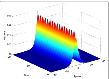
First, for the periodic problemμ= , we plot the waveform in Figure . One can observe that the nonstandard finite difference variational integrator () displays the numerical properties of the periodic solitary-wave clearly and precisely.
We define thel-errorekof the numerical solution at time steptkas
ek=
x
j uk
j –up(xj,tk).
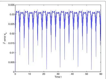
In Figure , we show thel-errorekof variational integrator () for the problemμ= .
Figure 1 The waveforms of()withμ= 1 by integrator().The waveforms of the NLSE with variable coefficients()(μ= 1) by the nonstandard finite difference variational integrator()witht= 0.1 and
Figure 2 l2-errore
kof integrator()for()withμ= 1.Numericall2-errorekof the nonstandard finite
difference variational integrator()for the NLSE with variable coefficients()(μ= 1), fromt= 0 tot= 60 witht= 0.1 andx= 0.1.
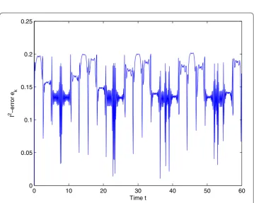
Now, we use the variational integrator () to solve the nonlinear Schrödinger equation () withμ= . Figure depicts the waveforms of the numerical solution obtained by the variational integrator (). Figure displays thel-errors of the variational integrator ().
4.2 Accuracy and numerical stability
To investigate the numerical convergence of the proposed scheme (), we conduct a series of numerical tests with varying mesh sizes. Thel-errors att= .,t= , andt= . are
listed in Table . The orders in the table are calculated with the formula [, ]
Order≈ln(Error(x)/Error(x)) ln(x/x)
.
Overall, it is clear that the error decreases as the mesh size goes to zero, indicating the con-vergence of our nonlinear integrator (). Moreover, the numerical orders clearly exhibit
second-order convergence when the mesh size decreases with fixingt= .x.
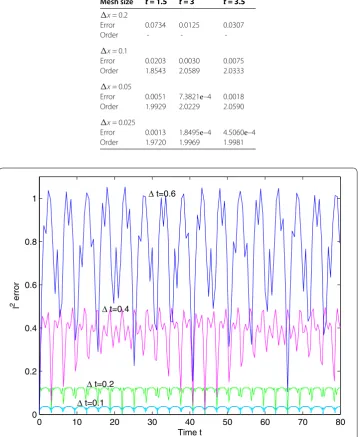
The numerical stability of the nonstandard finite difference variational integrator () is demonstrated in Figure .l-error curves are plotted with increasing time step sizes
t= ., ., ., ., respectively. We can see that our method performs very well even with large time steps and it is unrestricted by the CFL conditions []. Thel-errors are
Figure 3 The waveforms of()withμ= 2 by integrator().The waveforms of the NLSE with variable coefficients()(μ= 2) computed with the nonstandard finite difference variational integrator()with
t= 0.1 andx= 0.1.
Figure 4 l2-errore
kof integrator()for()withμ= 2.Numericall2-errorekof the nonstandard finite
Table 1 l2-errors and convergence orders of integrator()for the problemμ= 1 with
t= 0.1x
Mesh size t= 1.5 t= 3 t= 3.5
x= 0.2
Error 0.0734 0.0125 0.0307
Order - -
-x= 0.1
Error 0.0203 0.0030 0.0075 Order 1.8543 2.0589 2.0333
x= 0.05
Error 0.0051 7.3821e–4 0.0018 Order 1.9929 2.0229 2.0590
x= 0.025
Error 0.0013 1.8495e–4 4.5060e–4 Order 1.9720 1.9969 1.9981
Figure 5 l2-errore
kof integrator()with increasing time step sizes.Thel2-errors of integrator()for
the NLSE with variable coefficients()(μ= 1) with time step sizest= 0.1, 0.2, 0.4, 0.6, andx= 0.05.
4.3 Norm conservation laws
We know that the nonlinear Schrödinger equation has the following global norm conser-vation law:
R
|u|dx=constant.
The discrete version of this norm conservation law [] can be written as
Normk:=x
j
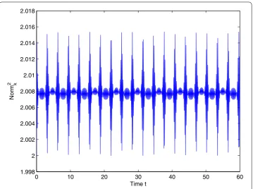
Figure 6 Norm conservation performance of integrator()for()μ= 1.Norm conservationNorm2 kof
the nonstandard finite difference variational integrator()for the NLSE with variable coefficients()(μ= 1), fromt= 0 tot= 60 witht= 0.1 andx= 0.1.
To show the performance of our integrator () on this aspect, we plot the norm
con-servation Norm
kin Figure and Figure . We find that our method preserves the norm
conservation law pretty well with very small periodic oscillation. The norm is constant within a percentage error of .% in Figure . For Figure , the norm is constant within a percentage error of %.
4.4 Comparison with standard finite difference methods
A numerical test is made to compare the nonstandard finite difference method with the standard finite difference method. For the nonlinear Schrödinger equation () withμ= , we have a standard finite difference scheme
iu k+
j –ukj t +αk+
uk+
j+ – ukj++ukj–+
(x) +βj+u
k+
j
ukj+= , ()
where the spatial and temporal derivatives are approximated by using the classical central differencing and the implicit Euler method, respectively.
Figure 7 Norm conservation performance of integrator()for()μ= 2.Norm conservationNorm2 kof
the nonstandard finite difference variational integrator()for the NLSE with variable coefficients()(μ= 2), fromt= 0 tot= 60 witht= 0.1 andx= 0.1.
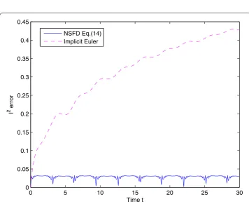
Figure 8 l2-error of the implicit Euler method()and the NSFD variational integrator().l2-error of the implicit Euler method()and the NSFD variational integrator()for the NLSE with variable coefficients
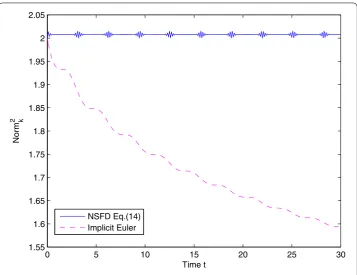
Figure 9 Norm2
kof the implicit Euler method()and the NSFD variational integrator().Norm2kof
the implicit Euler method()and the NSFD variational integrator()for the NLSE with variable coefficients
()(μ= 1).t= 0.1 andx= 0.1.
scheme,
iu k+
j –ukj t +αk+
(uk
j+– ukj +ukj–) + (ukj++– ukj++ukj–+)
(x)
+
βk+u
k j
+ukj+ukj +ukj+= ,
also has some flavor of the nonstandard finite difference method, i.e., discretizing
the equation at half time-grid points. The Crank-Nicolson scheme for the nonlinear Schrödinger equations also preserves the conservation law very well []; however, it is not multi-symplectic for the NLSE, which is a multi-symplectic PDE. We also compare
our method () with the Crank-Nicolson scheme here. From thel-errors shown in
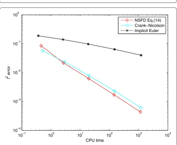
Fig-ure , we find both of them work well. To compare these two approaches in terms of computational efficiency, we perform a set of numerical tests with different spatial and temporal mesh sizes. Figure depicts thel-errors versus the computational time
con-sumed by each approach to achieve those errors. One can observe that our method is competitive to the Crank-Nicolson method in this case. What is more, our method costs less computational time to get error levels less than –.
Figure 10 l2-errors of the Crank-Nicolson scheme and the NSFD variational integrator().l2-errors of the Crank-Nicolson scheme and the NSFD variational integrator()for the NLSE with variable coefficients
()(μ= 1).t= 0.1 andx= 0.1.
Figure 11 Thel2-errors as a function of the CPU time for the NSFD variational integrator(),
5 Conclusion
In this paper, we have considered the nonlinear Schrödinger equation with variable coeffi-cients. We have derived two discrete variational integrators based on the nonstandard fi-nite difference methods, and have presented the corresponding discrete multi-symplectic structures via multi-symplectic form formulas. We have shown that it is feasible to com-bine the idea of discrete variational integrators and nonstandard finite difference methods to construct the multi-symplectic schemes for the NLS equation. The convergence and the stability of our methods have been discussed. The numerical experiments have shown the effectiveness and efficiency of these nonstandard finite difference variational integrators. Some comparisons with standard finite difference schemes have been made to demon-strate the features of the proposed integrators.
Competing interests
The authors declare that they have no competing interests.
Authors’ contributions
The authors declare that the study was realized in collaboration with the same responsibility. All authors read and approved the final manuscript.
Acknowledgements
We are grateful to the editor and anonymous reviewers for their careful reading and many constructive suggestions which led to a great improvement of this paper. This work is supported by the NNSF of China (No. 11271101) and the NNSF of Shandong Province (No. ZR2010AQ021).
Received: 15 October 2012 Accepted: 2 January 2013 Published: 16 January 2013
References
1. Zakharov, V, Manakov, S: On the complete integrability of a nonlinear Schrödinger equation. Theor. Math. Phys.19(3), 551-559 (1974)
2. Korepin, V, Bogoliubov, N, Izergin, A: Quantum Inverse Scattering Method and Correlation Functions. Cambridge University Press, Cambridge (1993). ISBN:978-0-521-58646-7
3. Hua, D, Li, X, Zhu, J: A mass conserved splitting method for the nonlinear Schrödinger equation. Adv. Differ. Equ. 2012, 85 (2012)
4. Ruffing, A, Meiler, M, Bruder, A: Some basic difference equations of Schrödinger boundary value problems. Adv. Differ. Equ.2009, Article ID 569803 (2009). doi:10.1155/2009/569803
5. Simon, M, Ruffing, A: Power series techniques for a special Schrödinger operator and related difference equations. Adv. Differ. Equ.2005(2), 109-118 (2005)
6. Karakashian, O, Makridakis, C: A space-time finite element method for the nonlinear Schrödinger equation: the discontinuous Galerkin method. Math. Comput.67(222), 479-499 (1998)
7. Delfour, M, Fortin, M, Payr, G: Finite-difference solutions of a non-linear Schrödinger equation. J. Comput. Phys.44(2), 277-288 (1981)
8. Feit, MD, Fleck, JA Jr., Steiger, A: Solution of the Schrödinger equation by a spectral method. J. Comput. Phys.47(3), 412-433 (1982)
9. Bridges, TJ: Multi-symplectic structures and wave propagation. Math. Proc. Camb. Philos. Soc.121(1), 147-190 (1997) 10. Hong, J, Liu, Y: A novel numerical approach to simulating nonlinear Schrödinger equations with varying coefficients.
Appl. Math. Lett.16(5), 759-765 (2003)
11. Hong, J, Liu, Y, Munthe-Kaas, H, Zanna, A: Globally conservative properties and error estimation of a multi-symplectic scheme for Schrödinger equations with variable coefficients. Appl. Numer. Math.56, 814-843 (2006)
12. Bridges, TJ, Reich, S: Numerical methods for Hamiltonian PDEs. J. Phys. A, Math. Gen.39, 5287-5320 (2006) 13. Reich, S: Multi-symplectic Runge-Kutta collocation methods for Hamiltonian wave equation. J. Comput. Phys.157(2),
473-499 (2000)
14. Bridges, TJ, Reich, S: Multi-symplectic integrators: numerical schemes for Hamiltonian PDEs that conserve symplecticity. Phys. Lett. A284(4-5), 184-193 (2001)
15. Hilscher, RS, Zeidan, V: Symmetric three-term recurrence equations and their symplectic structure. Adv. Differ. Equ. 2010, Article ID 626942 (2010). doi:10.1155/2010/626942
16. Zemánek, P: Rofe-Beketov formula for symplectic systems. Adv. Differ. Equ.2012, 104 (2012). doi:10.1186/1687-1847-2012-104
17. Zheng, B: Multiple periodic solutions to nonlinear discrete Hamiltonian systems. Adv. Differ. Equ.2007, Article ID 41830 (2007). doi:10.1155/2007/41830
18. Chen, J: A multisymplectic integrator for the periodic nonlinear Schrödinger equation. Appl. Math. Comput.170, 1394-1417 (2005)
19. Chen, J, Qin, M: Multi-symplectic Fourier pseudospectral method for the nonlinear Schrödinger equation. Electron. Trans. Numer. Anal.12, 193-204 (2001)
21. Chen, J, Qin, M, Tang, Y: Symplectic and multi-symplectic methods for the nonlinear Schrödinger equation. Comput. Math. Appl.43, 1095-1106 (2002)
22. Marsden, JE, West, M: Discrete mechanics and variational integrators. Acta Numer.10, 357-514 (2001)
23. Marsden, JE, Patrick, GW, Shkoller, S: Multisymplectic geometry, variational integrators, and nonlinear PDEs. Commun. Math. Phys.199(2), 351-395 (1998)
24. Mickens, RE: Application of Nonstandard Finite Difference Schemes, 1st edn. World Scientific, Singapore (2000) 25. Mickens, RE: Nonstandard finite difference schemes for differential equations. J. Differ. Equ. Appl.8(9), 823-847 (2002) 26. Mickens, RE: A nonstandard finite difference scheme for the diffusionless Burgers equation with logistic reaction.
Math. Comput. Simul.62, 117-124 (2003)
27. Mickens, RE: Dynamic consistency: a fundamental principle for constructing nonstandard finite difference schemes for differential equations. J. Differ. Equ. Appl.11(7), 645-653 (2005)
28. Mickens, RE: A numerical integration technique for conservative oscillators combining nonstandard finite-difference methods with a Hamilton’s principle. J. Sound Vib.285, 477-482 (2005)
29. Mickens, RE, Ramadhani, I: Finite-difference scheme for the numerical solution of the Schrödinger equation. Phys. Rev. A45(3), 2074-2075 (1992)
30. Vankerschaver, J, Liao, C, Leok, M: Generating functionals and Lagrangian PDEs. J. Math. Phys. (2012, submitted) 31. Ciarlet, PG, Iserles, A, Kohn, RV, Wright, MH: Simulating Hamltonian Dynamics. Cambridge Monographs on Applied
and Computational Mathematics. Cambridge University Press, Cambridge (2004)
32. Leok, M, Zhang, J: Discrete Hamiltonian variational integrators. IMA J. Numer. Anal.31(4), 1497-1532 (2011) 33. Arenas, AJ, González-Parra, G, Chen-Charpentier, BM: A nonstandard numerical scheme of predictor-corrector type
for epidemic models. Comput. Math. Appl.59(12), 3740-3749 (2010)
34. González-Parra, G, Arenas, AJ, Chen-Charpentier, BM: Combination of nonstandard schemes and Richardson’s extrapolation to improve the numerical solution of population models. Math. Comput. Model.52(7-8), 1030-1036 (2010)
35. Jordan, PM: A nonstandard finite difference scheme for nonlinear heat transfer in a thin finite rod. J. Differ. Equ. Appl. 9(11), 1015-1021 (2003)
36. Malek, A: Applications of nonstandard finite difference methods to nonlinear heat transfer problems. In: Heat Transfer - Mathematical Modelling, Numerical Methods and Information Technology (2011). doi:10.5772/14439 37. Ma, Q, Ding, D, Ding, X: A nonstandard finite-difference method for a linear oscillator with additive noise. Appl. Math.
Inf. Sci. (accepted)
38. Manning, PM, Margrave, GF: Introduction to non-standard finite-difference modelling. CREWES Research Report 18 (2006)
39. Zhou, S, Cheng, X: Numerical solution to coupled nonlinear Schrödinger equations on unbounded domains. Math. Comput. Simul.80, 2362-2373 (2010)
40. Zhou, S, Cheng, X: A linearly semi-implicit compact scheme for the Burgers-Huxley equation. Int. J. Comput. Math. 88(4), 795-804 (2010)
41. Courant, R, Friedrichs, K, Lewy, H: On the partial difference equations of mathematical physics. IBM J. Res. Dev.11(2), 215-234 (1967)
42. Che, C, Xue, X: Infinitely many periodic solutions for discrete second order Hamiltonian systems with oscillating potential. Adv. Differ. Equ.2012, 50 (2012)
doi:10.1186/1687-1847-2013-12