Indoor positioning based on statistical multipath channel modeling

(1)

R E S E A R C H

Open Access

Indoor positioning based on statistical multipath

channel modeling

Chia-Pang Yen

1*

and Peter J Voltz

2

Abstract

In order to estimate the location of an indoor mobile station (MS), estimated time-of-arrival (TOA) can be obtained at each of several access points (APs). These TOA estimates can then be used to solve for the location of the MS. Alternatively, it is possible to estimate the location of the MS directly by incorporating the received signals at all APs in a direct estimator of position. This article presents a deeper analysis of a previously proposed maximum likelihood (ML)-TOA estimator, including a uniqueness property and the behavior in nonline-of-sight (NLOS) situations. Then, a ML direct location estimation technique utilizing all received signals at the various APs is proposed based on the ML-TOA estimator. The Cramer-Rao lower bound (CRLB) is used as a performance reference for the ML direct location estimator.

Keywords:indoor positioning, maximum likelihood (ML), time-of-arrival (TOA), direct location estimation

1 Introduction

With the emergence of location-based applications and the need for next-generation location-aware wireless networks, location finding is becoming an important problem. Indoor localization has recently started to attract more attention due to increasing demands from security, commercial and medical services. For example, next generation corporate wireless local area networks (WLAN) will utilize location-based techniques to improve security and privacy [1]. The requirement for high accuracy positioning in complex multipath chan-nels and nonline-of-sight (NLOS) situations has made the task of indoor localization very challenging as com-pared to outdoor environments.

Conventionally, the positioning problem is solved via an indirect (two-step) parameter estimation scheme. First, the time-of-arrival (TOA) estimation at each access point (AP) is performed. The TOA estimator estimates the first arriving path delay, which corresponds to the line-of-sight (LOS) distance between the transmitter and the receiver assuming the LOS path exists. Then, these TOA estimates from each AP are transmitted to a central terminal at which the location estimation is carried out

by various algorithms, such as trilateration or least squares fitting, etc. [2,3]. Recently, the direct location estimation method has been proposed as another aspect to the positioning problem [4]. Unlike the indirect meth-ods which split the location estimation efforts between the APs and the central terminal, the direct positioning methods rely only on the central terminal to perform the location estimation task. The APs just relay the received signals to the central terminal for it to estimate the loca-tion of the mobile staloca-tion (MS). It has been shown that the direct method can outperform the indirect method [4].

For the indirect positioning methods, the first step is to obtain an accurate TOA estimation. To separate closely spaced channel paths, super-resolution techniques [5], such as multiple signal classification (MUSIC), etc. [6-8], are reported to be able to significantly improve the TOA estimations as compared to the conventional autocorrela-tion approach [9].

Maximum likelihood (ML) is a natural approach for TOA estimation but in order to resolve the multipara-meter issue that seems natural to the multipath environ-ments, a novel ML-TOA estimator that only requires a one-dimensional search is proposed in [10]. The ML-TOA technique estimates only the first arriving path delay based on the observation that this parameter is the only quantity needed for positioning. It was found that in * Correspondence: [email protected]

1

ITRI (Industrial Technology Research Institute), 195, Sec. 4, Chung Hsing Rd., Chutung, Hsinchu 310, Taiwan

Full list of author information is available at the end of the article

(2)

dense multipath environments, the ML-TOA estimation outperforms the super-resolution methods discussed in [11,12]. The effect of considering only the first arriving path delay in positioning was studied in [13]. Based on the analyses of the Cramer-Rao lower bound (CRLB), the authors showed that if the paths are correlated then including other paths could improve the TOA estimation accuracy, however, they also pointed out that doing so “would not help enhance the accuracy significantly but merely increase the computational complexity.”

In this article, several important properties pertaining to the ML-TOA estimator that were previously left unanswered are established. First is the uniqueness of the ML-TOA estimator. For TOA estimation in multi-path environments, not only the additive noise but also the multipath channels are random. Therefore, it is not obvious that the estimates converge to the exact para-meter when signal-to-noise ratio (SNR) increases. Here, we demonstrate that the ML-TOA estimation provides the unique, correct TOA in the absence of noise pro-vided the channel statistics are known. The effects of the NLOS situations are also discussed. The NLOS situation is another major challenge for indoor position-ing for it can cause large TOA estimation bias that in turn result in large location estimation errors [14]. There are optimization methods which can be used to mitigate the error due to NLOS. In [15,16], the optimi-zation is carried out with respect to the unknown mobile location or the NLOS bias. In [13,17,18], statisti-cal estimation methods are proposed in the case that the statistical knowledge such as the propagation scat-tering models or the NLOS delays statistics are known. In this article, the proposed ML-TOA is shown to be able to incorporate the statistics of NLOS channels automatically and thus reduce the estimation bias due to NLOS path delays.

The direct positioning method has just started to emerge as an interesting research topic and has been shown to provide improvement in the location estimation accuracy. Thus, in this article, in addition to the indirect (two-step) method, we also propose a direct ML position-ing algorithm based on the ML-TOA estimator. In [19], the authors proposed a direct positioning method for orthogonal-frequency-division-multiplexing (OFDM) sig-nals. There, the APs are assumed to be equipped with antenna arrays, the source is located in the far field and the channel power delay profile has a significant path while the rest paths are ignored. Here, we assume that each AP has a single antenna and the channel has multi-path. It is shown that our proposed ML direct location estimator also posesses the uniqueness property thus its estimates are reliable. Furthermore, the CRLB of the direct location estimator is used as a performance refer-ence. The simulation results show that the proposed

direct positioning method has better performance than the indirect method and is close to the CRLB for some channels. While we focus on an OFDM signal structure, which is mathematically convenient and has not been studied extensively in the indoor localization problem, the approach can be generalized to any signal type.

The remainder of the article is organized as follows. Section 2 presents the mathematical formulation of the TOA estimation problem and the ML-TOA estimator. Section 3 presents analyses of the proposed ML-TOA estimator including the uniqueness property, the beha-vior of the cost function and the effects of the NLOS situations. In Section 4, a ML direct positioning algo-rithm is proposed based on the ML-TOA estimation algorithm. The uniqueness property associated with the ML direct location estimator is also shown. In Section 5, the performance of ML-TOA estimator and the pro-posed direct algorithm are demonstrated through com-puter simulations. Finally, conclusions are presented in Section 6.

2 ML-TOA estimation

One OFDM symbol duration isT+TG, whereTGis the guard interval, andTis the receiver integration time over which the sub-carriers are orthogonal. A single symbol of the transmitted OFDM signal is assumed to haveN sub-carriers with transmitted sequence vectord= [d0d1· · ·

dN-1]T. Assume that the signal is received after passing through a multipath channel with impulse response h(t) =L_i₌₀−1aiδ (t−τi) in which 0≤τ0≤τ1≤· · ·≤τL-1 ≤TGandaiis the complex channel gain of theith path. After the standard receiver sampling, guard interval removal and fast-Fourier-transformation (FFT) proces-sing, thekth element of the FFT output vector is (see [10] for details)

where nk is complex Gaussian noise with variance s2

=N0.

Conventional ML estimation is formulated in such a way that the unknown parameter is a multivariate vec-tor, i.e.,θ = [a0 ...aL-1τ0...τL-1]T. When the number of pathsL is large, the computational complexity becomes prohibitive. However, only the first path delay, τ0, is required for location estimation purpose. Therefore, we focus the ML estimation on the TOA only, assuming a statistical model of the channel.

(3)

other path delays can be written as

zero delay frequency response at thekth subcarrier. Define the subcarrier frequency response vector ash= [H0 H1 ...HN-1]T. We assume at first that h is a zero mean, circular complex Gaussian vector with known

covariance matrixKh=E

hhH

, where the Hdenotes Hermitian transpose [20]. This Gaussian assumption is for mathematical development and the proposed TOA estimator, as was demonstrated in [10] for Ray-Trace data, performs well in practical situations. Equation (2) can then be used to express the complete FFT output vector as symbols. We shall assume that time delay estimation is performed on an OFDM training symbol so that D is known. As shown in [10], the ML solution for TOAτ0is

where the cost function of the estimator is defined as

Q(τ)yHG(τ)FG(τ)Hy, (5)

whereF =DR(s2I+RHDH DR)-1RHDHandRis a rankL(< N) factor ofKh asKh=RRH.

3 Performance characteristics of the ML-TOA estimator

When estimating TOA in a dense multipath environ-ment, the accuracy is impacted not only by the noise, but also by the presence of the many echoes of the sig-nal due to the multipath. In this section, we first demonstrate that when noise is absent and we are in the presence of multipath only, then the proposed esti-mator yields the correct TOA uniquely, provided the covariance matrixKh is exactly known. For the rest of

the article, we assume that D = I without loss of generality.

3.1 Uniqueness of the ML-TOA estimation

Assume for the present that noise is absent, i.e.,s2 = 0. Since Kh can be factored using the Singular Value

DecompositionKh= (UΛ1/2UH) (UΛ1/2UH) = RRH, the

channel can be expressed as

h=Rz, (6)

wherezÎCLis a zero mean Gaussian random vector with covariance matrix {zzH_}₌_I _and_L_{is the rank of} Kh. In this case, the received FFT output vector will be

y=G(τ0)h =G(τ0)Rz.

Using this expression and the fact that when noise is absent the F matrix reduces to F =R(RHR)-1 RH and identity matrix. We would like to investigate whether there are other possible maximizing values ofτ.

To simplify the notation, let θ = 2_Tπ(τ−τ0) and defineG(θ)≜GH(τ- τ0). We are looking for conditions on θ such that G(θ)Rz Î Range(R), θ = 0 being an obvious solution. We note first that we can convert this problem into the deterministic one of finding conditions on θ such that Range (G (θ) R)⊆ Range(R). Certainly this latter condition is sufficient to guarantee that G(θ) RzÎ Range(R). It is also true that if Range (G(θ)R)⊈ Range(R), then G(θ)Rz∉Range(R) with probability one. To see this, note that Range (G(θ)R) ⊈ Range(R) is equivalent to [Range (R)]⊥⊈[Range (G(θ)R)]⊥where⊥ denotes the orthogonal complement. Letv denote any non-zero vector such that v Î [Range (R)]⊥ but v ∉ [Range (G(θ)R)]⊥. Then,vHG(θ)R≠0 and the random variablevHG(θ)Rzis Gaussian with non-zero variance and will be non-zero with probability one. Therefore, with probability one, vH G(θ)Rz ≠ 0 and G(θ)Rz ∉ Range(R) because it is not orthogonal tov.

Now, the deterministic condition Range (G(θ)R) ⊆ Range (R) is equivalent to the existence of some matrix Asuch that G(θ)R =RA. Multiplying on the left byG the structure ofG, we see that

(4)

Equation (7) says that any matrix of the form (8) can multiply Ron the left, and the resulting matrix f(G)R satisfies Range (f(G)R)⊆Range (R).

Let us now assume that Range(R) includes the flat channel vectorhf =1where1is a vector with all unit elements. This essentially assumes that a flat fading channel is one of the possible realizations so that there is a vector z such that 1 = Rz. Multiplying (7) by z yieldsf(G)1=Rf(A)zwhich means that, from (6),

f(G)1=f(1) f(ejθ) f(ej2θ) · · · f(ej(N−1)θ)T (9)

is a realizable channel vector for any polynomialf(l). Now, let Lbe the rank of Rand assume that L < N. Then, theN values {1,ejθ, ej2θ,...,ej(N-1)θ} cannot all be distinct for, if they were, the channel vector (9) could be chosen arbitrarily by suitable choice of interpolating polynomial f(l), contrary to the fact that the realizable channels are restricted to the L dimensional space Range (R). This is due to the well-known fact that a polynomial can always be found, which takes arbitrary values on any given set of arguments. In fact, we can see that at most Lof the values {1, ejθ, ej2θ,...,ej(N-1)θ} can be distinct for a similar reason. Now suppose there are actually q distinct values. It follows that the firstq

values must be distinct because, for example, if ejrθ =

ejpθwhere r < p≤q then ej(p-r)θ = 1 and there will be onlyp-r- 1< qdistinct values.

We have now shown that there must be an integer

q ≤ L such that ejqθ = 1. Then, the sequence {1, ejθ,

ej2θ,...,ej(N-1)θ} cycles as follows {1, ejθ, ej2θ,..., ej(q-1)θ, 1,

ejθ, ej2θ,...}. Suppose for example thatq = 2. Then, the sequence is {1,ejθ, 1, ejθ,...,1,ejθ,...}. Choose an interpo-lating polynomial such that f(1) = 1 and f(ejθ) = -1. Then, from (9) the vector of alternating plus and minus ones, i.e.,f(G)1= [1 -1 1 -1 1...]T would be a realizable channel vector. But this highly oscillatory channel fre-quency response would imply a very large channel delay spread. Therefore, if the delay spread of the channel is not too large, the value q = 2 would not be realistic. Similar examples of unrealistic channel frequency response can be constructed for anyq greater than 1. Therefore, we are left withq= 1 in which case the only solution is ejqθ = 1 so that θ = 0 and the solution is unique. The simulation results in Section 5.1 also demonstrate this uniqueness property of the ML-TOA estimator.

3.2 ML-TOA estimation in NLOS situations

In this section, the effect of NLOS on the ML-TOA esti-mator is discussed and we show that the NLOS case is very naturally incorporated into the proposed ML-TOA estimator. Recall (1), (2) and (3) which illustrate how

the TOA τ0 is factored out and incorporated into theG matrix. These equations were developed with the under-standing thatτ0 was the path delay of the direct LOS path. From now on, however, we simply define TOAτ0 as the time it would take for an electromagnetic wave to travel the straight line that links the MS and AP, whether or not such a direct LOS path actually exists. In the case when a LOS path does not exist, (1) would be modified to read

yk=dk

where thei= 0 term has been removed since the LOS path is absent. Nevertheless, withτ0 defined as above, we may still express the actual path delays in terms of

τ0 as τi=τ0+ (τi−τ0) =τ0+τ¯i, and we obtain a

modi-the zero delay frequency response at modi-the kth subcarrier when no LOS path is present. We maintain the earlier definition of the subcarrier frequency response vector as h = [H0 H1 ... HN-1]T and (11) can be used to express the complete FFT output vector as

y=G(τ0)Dh+n. (12)

Note that (12) is exactly the same as (3). The only dif-ference in this NLOS case is the modification of the ele-ments of the h vector due to the absence of the direct path. The derivation of the ML estimator now follows exactly as the case in which a direct path is present, and the channel statistics as measured by the procedure out-lined below will reflect the actual environment, whether or not there is always a direct path present.

In practice, no matter what the multipath structure, the channel covariance matrixKh can be estimated

off-line by averaging measurements at each AP while the MS transmits at some known locations chosen in a ran-dom fashion. The detailed procedure is as follows: Step 1 : For a given, known, AP location, measure the received FFT output vectory(i)at the AP for theith MS location.Step 2: Since, in this measurement phase, both MS and AP locations are known, TOA of the ith MS transmission (atith location), i.e., _τ₀(i), can be computed by dividing the distance between them by the speed of light, and the G(i) matrix can be determined by

(5)

Then, for this ith transmission, the FFT output vector y in Equation (12) is measured and an estimated

snapshot of h(i) can be found by

h(i)= (G(i))−1y(i)₌_h(i)_{+ (}_G(i)₎−1_n(i)_._{Step 3}_{: After} col-lecting measurements atP different MS locations, the estimated channel covariance matrix is obtained by

ˆ

For future reference we now define the NLOS delay. For the NLOS case in which a LOS path does not exist,

τ1 in (10) will be the first arriving path delay. Then, we define “NLOS delay” =τ1 - τ0, where τ0 is the line of sight distance divided by the speed of light, as described above. The NLOS delay is sometimes called the excess delay and is the time difference between the first arriv-ing actual NLOS path and the direct LOS time delay,τ0.

At this point, we emphasize that the NLOS case is very naturally incorporated into the proposed ML-TOA estimator. Recall that in the entire development, includ-ing the estimation procedure for Kˆh above, TOA is defined as the time it takes for the electromagnetic waves to travel the straight line that links the MS and AP, whether or not such a LOS path actually exists. Therefore, inStep 2 above the TOA can still be com-puted given the location of MS and AP even in the absence of a LOS path, since TOA is known whether or not a direct LOS exists. This is based on the idea that motivates the ML-TOA estimation. That is to separate the desired parameter from the statistics of the multi-path channel. For the purpose of positioning, the desired parameter is the“generalized” TOA that we defined in the beginning of this section. In this way, the statistical properties of the measured channels will naturally incor-porate the NLOS properties of the channel and no extra step or a priorinformation about the NLOS statistics is required to mitigate the NLOS effects. In Section 5.1, we present simulation results which show the TOA esti-mation performance for both LOS and NLOS cases. Finally, we point out that, since (12) is identical to (3), the uniqueness proof in Section 3.1 applies to the NLOS case as well.

3.3 Properties of the cost functionQ(τ)

The TOA estimation is a nonlinear problem and is known to exhibit ambiguities which could result in large errors [21,22]. In the large error regime, the CRLB can-not be attained. In this section, the behavior of the cost functionQ(τ) is studied for two multipath channel mod-els. It is also shown that for single path channels, the ML-TOA estimator is unbiased and the estimation error variance is inversely proportional to the bandwidth.

Consider first the extreme case in which there is only a direct path atτ0 = 0 and no additive noise. We haveh

wherea,b are some constants. The width of the main lobe is inversely proportional to the number of subcar-riersNor equivalently the bandwidth. In Figure 1, one realization of the noise free cost functionQ(τ) in a sin-gle path channel is shown for the 802.11a configuration whereN= 64 (see Section 5). It can be seen that it clo-sely matches the theoretical curve where the training sequence is assumed to be all 1’s.

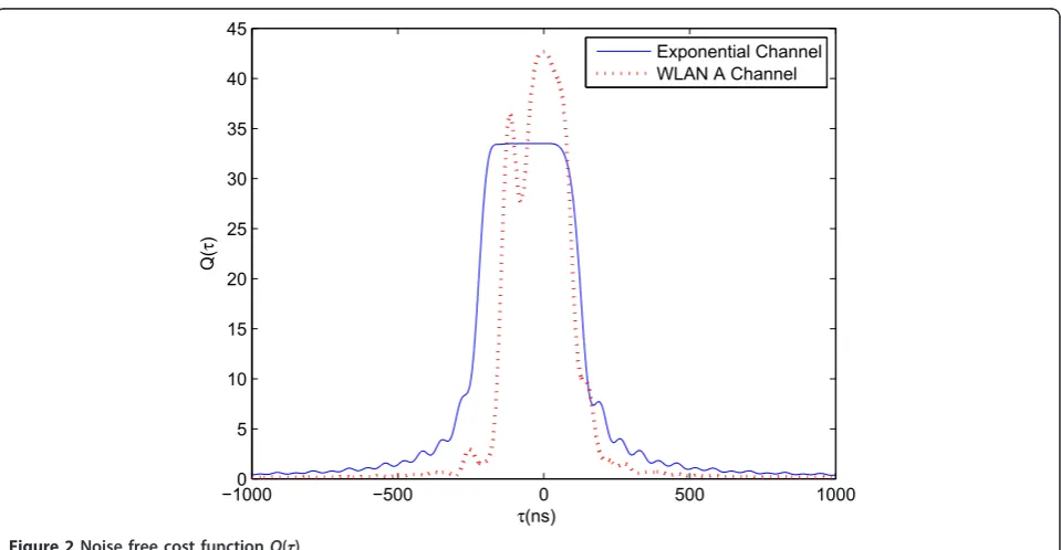
In the case of multipath, we first investigate the cost functionQ(τ) when noise is absent. In Figure 2, one rea-lization of the noise free cost function for Exponential channel model and WLAN channel model A (see Sec-tion 5 for detailed descripSec-tion of the channel models used in this article) are plotted. Note the noise free cost function for the Exponential channel is fairly flat. As demonstrated in Section 3.1 ifKhis perfectly known the

actual peak of the cost function is at zero offset, but at high SNR, where the flattening effect is observed, an error in Kh can result in biased TOA estimation (see

Figure 3). The noise free cost function for WLAN chan-nel model A shows that a clear peak is present thus is more robust to the error from the estimated channel covariance matrix at high SNR region (see Figure 4). For all other WLAN channel models, i.e., B to D, we have observed that the cost functions have similar character-istics to those for channel model A.

4 ML direct positioning method

In this section, we develop a ML direct estimation of the MS position, (x,y), based on the received FFT vectors from several APs. The proposed ML direct location esti-mation is shown to provide the correct, unambiguous location in the absence of noise given the channel statistics.

(6)

estimator described in Section 2, to estimate the position of MS directly.

For simplicity, in this article, the MS location is assumed to be on a two-dimensional surface, but the derivation can be extended to three dimensions as well. ConsiderMAPs located at heightzabove the MS withx,

y locations (xi, yi) (i = 1, 2,..., M) and an MS at an unknown location (x, y). The distance from the MS to

theith AP is thendi=

(x−xi)2+ (y−yi)2+z2.

There-fore, the TOA from the MS to the ith AP is

τ(i) 0 =dCi =

(x−xi)2+ (y−yi)2+z2

C

, where C is the

speed of light. Notice that in this expression, the TOA τ(i)

0 is a function of the unknown position of MS, i.e.,

í10000 í500 0 500 1000

0.2 0.4 0.6 0.8 1 1.2 1.4 1.6 1.8

τ (ns)

Q(

τ

)

Theoretical 802.11a

Figure 1Noise free cost functionQ(τ) for single path channel.

í10000 í500 0 500 1000

5 10 15 20 25 30 35 40 45

τ(ns)

Q(

τ

)

Exponential Channel WLAN A Channel

(7)

(x,y). We can estimate the position of the MS directly, based on the FFT output vectors at allMAPs as follows.

From (3), assuming D= I, the complete FFT output vector at theith AP is

y(i)=G(i)h(i)+n(i), (13)

where G(i)_{= diag}

1,e−j

2π CT √

(x−xi)2+(y−yi)2+z2

,. . .,e−j(N−1)

2π CT √

(x−xi)2₊₍_y₋_yi₎2₊_z2

.

The noise vectorsn(i)are independent, zero mean Gaus-sian with covariance matrix σ_i2I andh(i)is assumed to be a zero mean, circular complex Gaussian vector with

known covariance matrix K(_hi)=

h(i)

H . The

0 10 20 30 40 50 60 70 80

í15

í10

í5 0 5 10 15 20

SNR (dB)

Mean of TOA estimation error (ns)

Exact K_h Mismatched K_h

Figure 3Performance comparisons between estimations using exact and mismatched covariance matrix Khfor the Exponential

channel model.

í5 0 5 10 15 20 25 30 35

í10 í8 í6 í4 í2 0 2 4 6 8 10

SNR (dB)

A Channel B Channel D Channel E Channel

(8)

channels from the MS to each AP are assumed to be independent. Then, the joint p.d.f. of the received FFT vectors from all APs is

p(y(1)_,_y(2)_,_{. . .,}_y(M)_|₍_x_,_y_{)) =} 1

where Det(·) denotes the matrix determinant and

K(yi)= each determinant factor inside the product can be

expressed as

i ) which does not depend

on (x,y).

Use this in (15) and define

Q(i)(x, y) 1

where the unknown parameter (x, y) is embedded in G(i). Note thatF(i)can be computed off-line given σ2 i

and K(_hi).

Next, we show that the ML direct positioning estimate based on (18) is unambiguously correct in the absence

of noise. Denote (x0,y0) and τ₀(i) the true location of the MS and the true TOA for theith AP, respectively. From the uniqueness property shown in Section 3.1, it follows

that, given i, Q(i)₍_τ(i)_{) =} 1

Assume that the ML direct location estimate is not unique. Then, from (18), there exists (x, y) ≠(x0, y0)

However, from the uniqueness property, it follows that

Q(i)(x0, y0) =Q(i) tem of equations are satisfied:

τ(i)

However, by the trilateration principle that is com-monly used in positioning, this cannot be true whenM ≥ 3 and thus a contradiction. Therefore, the proposed ML direct position estimate is unique.

5 Simulation results

(9)

dB for each path. The channel covariance matrix Kˆh is estimated using the procedures described in Section 3.2 with 100 samples and 40 dB received signal SNR. The received SNR is defined as, assuming the transmit signal power is unity, SNR {iL=0−1|a

2

i|}

σ2 .

5.1 Performance of the ML-TOA estimator

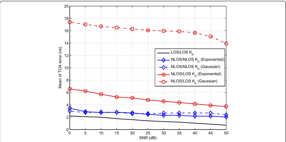
The performance of the ML-TOA estimator described in Section 2 has been thoroughly presented in [10] in the case when there is a significant LOS path present. In this section, we first discuss its performance in NLOS channels and then consider the effects of matched vs. mismatched statistics. As discussed in Section 3.2, the ML-TOA esti-mation procedure takes the statistics of NLOS channels into account automatically. Recall that the term“NLOS delay”refers to the time difference between the first arriv-ing path delay and the TOA as defined in Section 3.2. If a direct LOS path exists, the NLOS delay is zero. Gaussian and Exponential distributions are assumed for the NLOS delay in the simulations [31,32]. In Figure 5, the NLOS delay is assumed to be Gaussian with mean 15 ns and var-iance 10 or Exponential with meanb= 3 ns. The bottom curve (LOS/LOSKh) is the performance when the LOS

path exists. The curves (NLOS/NLOSKh) are the

situa-tions when the channel contains no LOS path. The curves (NLOS/LOSKh) serve as references and they represent a

NLOS case but when estimating Kˆh,τ0(i) is chosen to equal the first arriving path delay instead of the TOA. The figure shows that the NLOS performance is comparable to that of the LOS case when channel measurements are made in the same NLOS scenario. If the LOS covariance matrix is used in the NLOS case (NLOS/LOSKh),

how-ever, an increased bias is seen.

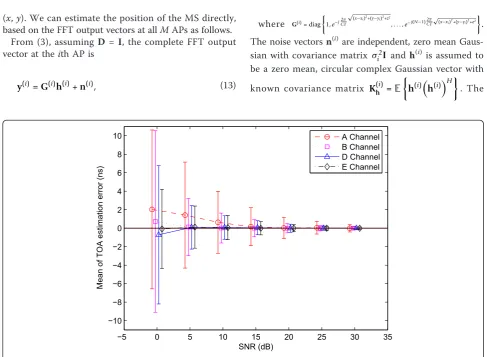
Next, we compare the performance of the ML-TOA estimator when the Exponential channel model is used vs. when the WLAN channel models are used, and also discuss the dependence of its performance on the num-ber of samples used in estimating the covariance matrix. The error-bar plot is used in Figures 3 and 4. The center

of the error bar is the mean of the estimation error and the length of the bar equals twice the standard deviation. In order to make it easier to distinguish different curves in the error-bar plot, they are off-set in the horizontal axis deliberately. These statistics are computed after 10, 000 trials. Figure 3 shows the performance of the ML-TOA estimator for the Exponential channel in the case where a LOS path exists. In order to show the robustness of the ML-TOA estimator, we compare the cases of mis-matched and mis-matched statistics. In the mismis-matched case, which corresponds to the practical application, the esti-mated covariance matrix Kˆh is measured as in Section 3.2 using 100 averaged samples. For the matched covar-iance matrix case, the channel is generated byh=Rzto ensure that its covariance matrix is strictly equal toKh.

From Figure 3, we can see that in the SNR range 0-40 dB, the estimation errorΔKhdoes not cause much

per-formance degradation for the Exponential channel. At high SNR region, as discussed in Section 3.3, due to the flattening of the cost function,ΔKhresults in biased

esti-mates. From the performance of the matched case, it is seen indirectly that the cost function has a unique maxi-mizer, for at high SNR, the estimation is unbiased and the variance is zero.

For the WLAN channel models, Figure 4 shows the performance for different channel types. By comparing Figure 4 with Figure 3, it seems that the performance for the WLAN channel models is slightly better than for the Exponential channels. This is related to the fact that, for these channels, the cost function has clear peak (see Fig-ure 2). Channel type A yields worst performance among the WLAN channels, which may be due to the fact that its power delay profile is most similar to an Exponential channel which has a flat noise free cost function.

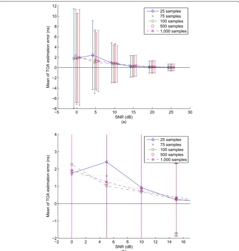
Figure 6 shows the performance of the WLAN chan-nel A as the number of samples used for estimatingKh

is varied. Since Kˆh is a random quantity for any given number of samples, we use the following process in gen-erating this figure. When the number of samples is P,

ˆ

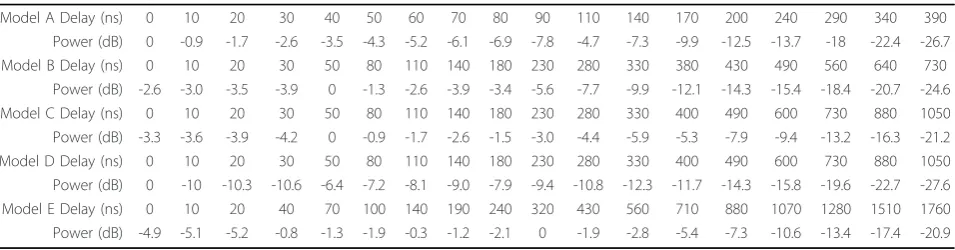
Kh is estimated usingPaveraged random channels (MS Table 1 Power delay profiles for the WLAN channels

Model A Delay (ns) 0 10 20 30 40 50 60 70 80 90 110 140 170 200 240 290 340 390

Power (dB) 0 -0.9 -1.7 -2.6 -3.5 -4.3 -5.2 -6.1 -6.9 -7.8 -4.7 -7.3 -9.9 -12.5 -13.7 -18 -22.4 -26.7

Model B Delay (ns) 0 10 20 30 50 80 110 140 180 230 280 330 380 430 490 560 640 730

Power (dB) -2.6 -3.0 -3.5 -3.9 0 -1.3 -2.6 -3.9 -3.4 -5.6 -7.7 -9.9 -12.1 -14.3 -15.4 -18.4 -20.7 -24.6

Model C Delay (ns) 0 10 20 30 50 80 110 140 180 230 280 330 400 490 600 730 880 1050

Power (dB) -3.3 -3.6 -3.9 -4.2 0 -0.9 -1.7 -2.6 -1.5 -3.0 -4.4 -5.9 -5.3 -7.9 -9.4 -13.2 -16.3 -21.2

Model D Delay (ns) 0 10 20 30 50 80 110 140 180 230 280 330 400 490 600 730 880 1050

Power (dB) 0 -10 -10.3 -10.6 -6.4 -7.2 -8.1 -9.0 -7.9 -9.4 -10.8 -12.3 -11.7 -14.3 -15.8 -19.6 -22.7 -27.6

Model E Delay (ns) 0 10 20 40 70 100 140 190 240 320 430 560 710 880 1070 1280 1510 1760

(10)

locations) with SNR at 40 dB. Next, using this specific ˆ

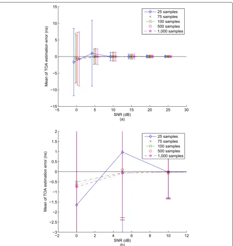
Kh, 100 random ML-TOA estimation trials are per-formed for each SNR value and the errors are recorded. Next, a new Kˆh is generated using anotherP averaged samples, and another 100 random ML-TOA estimation trials are performed for each SNR value. This is repeated for 10 different estimated Kˆh matrices, for a total of 1, 000 TOA estimation error values, and the sta-tistics are then plotted to yield the curves in Figure 6. Figures 7 and 8 show the corresponding results for the WLAN channel D and Exponential channel. As one would expect, there is some fluctuation in the curves, which decreases with increasing P, but forP ≥100 the curves track each other fairly closely. For the remainder of the article, P = 100 is used in the simulations presented.

Table 2 presents some error statistics forKhitself. For

each value ofP(number of averaged samples) the table shows the maximum (over all elements of Kˆh) of the normalized RMS error in the elements of Kˆh over 1, 000 random estimates. The error is the difference between Kˆh and the “true” covariance matrix as esti-mated using 10, 000 samples. Then, the normalization is obtained by dividing the RMS error in each element by the magnitude of the“true” covariance matrix. In prac-tice, for a given indoor environment, an initial estima-tion of Kh would be carried out off-line prior to the

employment of the ML-TOA procedure for localization. Subsequent additional measurements for this purpose

could then be added later to improve the estimation accuracy if necessary.

5.2 Performance of ML direct positioning

We compare the performance of two localization schemes. One is the proposed ML direct location tech-nique discussed in Section 4. The other is an indirect (two-step) method which first uses the ML-TOA mation approach described in Section 2 for TOA esti-mates then least square localization solvers described in [3], namely the least square (LS) and TOA-weighted constraint LS (TOA-WCLS) techniques, are adopted to solve for the location of the MS. The least square localization solvers can be used with any TOA estimation technique for the individual AP’s, but here we use the ML-TOA estimation approach described in Section 2 so that both techniques have the benefit of the measured channel statistics. A five AP geometry is considered in a 100 m× 100msquare with AP coordi-nates; (5, 10), (50, 50), (80, 20), (10, 75) and (90, 90), respectively. We show results for three MS locations, namely at (x, y) = (20, 20), (20, 90) and (70, 70). The channel impulse responses for each of the five APs are generated randomly using the aforementioned channel models.

In the simulations, the average SNR is defined as 1

M

i=1SNRi, where SNRi is the signal-to-noise power ratio at the ith AP. The path loss exponent is assumed to be 3 for indoor environments. The weighting matrix W used in TOA-WCLS is then chosen such that the

0 5 10 15 20 25 30 35 40 45 50

0 2 4 6 8 10 12 14 16 18 20

SNR (dB)

Mean of TOA error (ns)

LOS/LOS K_h

NLOS/NLOS K_h (Exponential)

NLOS/NLOS K_h (Gaussian)

NLOS/LOS K_h (Exponential)

NLOS/LOS K_h (Gaussian)

(11)

diagonal elements are wii= MSNRi

i=1SNRi. The results shown here are obtained by running 10,000 random trials.

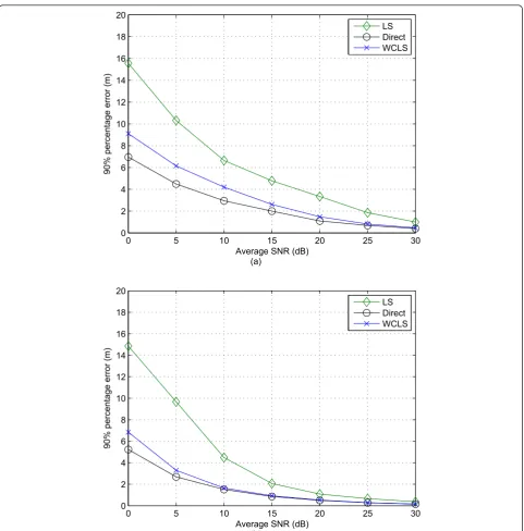
Figures 9 through 12 are for MS location at (x, y) = (20, 20). Figures 9 and 10 show the performance com-parisons between the direct method and the indirect (TOA-LS and TOA-WCLS) methods for the Exponen-tial channel models. Figure 9 shows the 90% percentage

error values versus average SNR. The 90% percentage error value is the value such that 90% of all errors are less than that value. As expected, the direct method out-performs the TOA-LS and TOA-WCLS methods, and the TOA-WCLS performs better than the TOA-LS, which imposes no weighting constraint. For the Expo-nential channel model, it is seen that due to the bias of the TOA estimations, the direct and indirect methods

í5 0 5 10 15 20 25 30

í8

í6

í4

í2 0 2 4 6 8 10 12

SNR (dB) (a)

25 samples 75 samples 100 samples 500 samples 1,000 samples

í2 0 2 4 6 8 10 12 14 16

í2

í1 0 1 2 3 4

SNR (dB) (b)

(12)

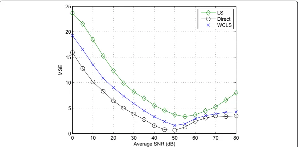
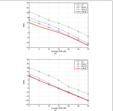
do not converge at high SNR, with the direct method maintaining its superiority. This is one rationale behind using the direct method. Figure 10 shows the mean square error (MSE) of the direct and indirect methods. Again, it is seen that the direct method has the best per-formance. Figures 11 and 12 show the performance with WLAN channel models A and D. Since the ML-TOA estimates of WLAN channels are unbiased when SNR is

high (see Figure 4), we do not show the performance at very high SNR for the performance converges. Figure 12 illustrates the CRLB as a performance reference for the WLAN channels. The CRLB is a lower bound on the variance of any unbiased estimator. Thus, we show it as a performance reference for the WLAN channels. The expressions for the CRLB can be found in Appendix A (due to limited space the detailed derivation is omitted).

í5 0 5 10 15 20 25 30

í15

í10

í5 0 5 10 15

SNR (dB) (a)

í2 0 2 4 6 8 10 12

í3

í2.5

í2

í1.5

í1

í0.5 0 0.5 1 1.5 2

SNR (dB) (b)

(13)

When computing the CRLB, each estimated channel covariance matrix K(_hi) is obtained by time-averaging 10, 000 random generated channels. The direct method again shows the best performance. Furthermore, the ML direct method is shown to have performance close to the CRLB. One can see that the performance for the

í5 0 5 10 15 20 25 30

í20

í15

í10

í5

0 5 10 15 20 25

SNR (dB) (a)

4 6 8 10 12 14 16 18 20 22

í3

í2

í1

0 1 2 3 4 5

SNR (dB) (b)

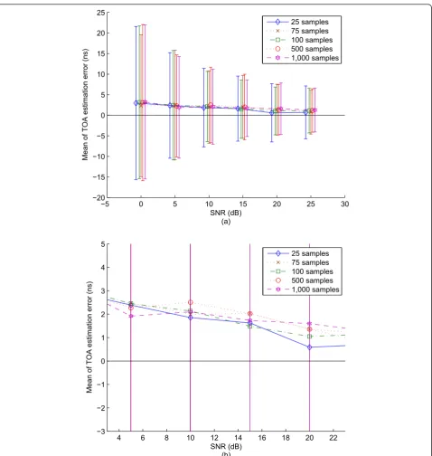
Figure 8Exponential channel: (a) TOA estimation error with respect to number of averaged samples for Kh; (b) expanded scale.

Table 2 Khestimation error statistics

Samples Max. normalized RMS error

25 1.422 × 10-2

100 3.347 × 10-3

500 2.614 × 10-3

(14)

WLAN model is better than for the Exponential model due to biased ML-TOA estimates in the latter. Figures 13 and 14 show the performance comparisons in WLAN channel model A for MS at (20, 90) and (70, 70). These two figures show results consistent with Fig-ures 11 and 12.

6 Conclusions

Several important results regarding the ML-TOA esti-mator for dense multipath indoor channels have been established. First, the unambiguous accuracy of the ML-TOA solution is proved in the noise free case, when multipath is the only detrimental effect of the channel.

0 10 20 30 40 50 60 70 80

0 5 10 15 20 25

Average SNR (dB)

90% percentage error (m)

LS Direct WCLS

Figure 990% percentage error for direct and indirect (two-stage) methods using Exponential channel model.

0 10 20 30 40 50 60 70 80

0 5 10 15 20 25

Average SNR (dB)

MSE

LS Direct WCLS

(15)

Then, the behavior in the NLOS case was discussed. Because of its statistical basis, the ML-TOA technique automatically incorporates the NLOS case in which there does not actually exist a direct path from the AP to the MS. The performance of the ML-TOA estimator was also detailed. It was shown that for single path channels, the ML-TOA estimator is unbiased and the estimation error variance is inversely proportional to the bandwidth. For multipath channels, the error is

dependent upon the specific characteristics of the chan-nels. Finally, we have shown how to extend the statisti-cal channel model (ML-TOA) approach to a direct ML localization technique which enables us to obtain a ML estimator that directly estimates the location of the MS. Results were compared to an indirect approach in which TOA estimates are obtained by the ML-TOA estimator and a least squares technique is then used to localize the MS. The direct ML location estimation is shown to

0 5 10 15 20 25 30

0 2 4 6 8 10 12 14 16 18 20

Average SNR (dB) (a)

LS Direct WCLS

0 5 10 15 20 25 30

0 2 4 6 8 10 12 14 16 18 20

Average SNR (dB) (b)

LS Direct WCLS

(16)

outperform the indirect methods and obtain perfor-mance close to the CRLB for some channel types.

Appendix A: Cramer-Rao lower bound for the ML direct position estimator

For the position estimation problem in which the unknown parameter isu = [x y]T, Fisher’s Information

Matrix [33] is given by

I(u) = –

From (14) and the well-known identity tr(AB) = tr (BA), the elements of the Fisher’s information matrix are given by

(17)

and

_∂2_ln_p₍_y_|_u₎

∂x∂y = M

i=1

2 σ2

i

Re

tr

D(xyi)C(Ri)+D

(i)

xC(Ri)(D

(i)

y) H

K(yi) , (23)

where D(xi)= diag

0,−j2π(x−xi) CdiT ,−2j

2π(x−xi)

CdiT ,. . .,−(N−1)j

2π(x−xi) CdiT

,

D(yi)= diag

0,−j2π(_Cdy−yi)

iT ,−2j 2π(y−yi)

CdiT ,. . .,−(N−1)j 2π(y−yi)

CdiT

,

0 5 10 15 20 25 30

0 2 4 6 8 10 12 14 16 18 20

LS Direct WCLS

0 5 10 15 20 25 30

í20

í15

í10

í5 0 5 10 15 20 25

MSE

LS Direct WCLS CRLB

(18)

D(ci)= diag

0,−j2π

CdiT,−j2

2π

CdiT,. . .,−j(N−1)

2π CdiT

,D(xyi)=Dx(i)D(yi),CR(i)=G(i)F(i)(G(i))H

and Re (·) denotes the real part of the argument.

Author details 1

ITRI (Industrial Technology Research Institute), 195, Sec. 4, Chung Hsing Rd., Chutung, Hsinchu 310, Taiwan2_{Electrical and Computer Engineering}

Department, Polytechnic Institute of New York University, Six MetroTech Center, Brooklyn, NY 11201, USA

Competing interests

The authors declare that they have no competing interests.

Received: 17 February 2011 Accepted: 30 November 2011 Published: 30 November 2011

0 5 10 15 20 25 30

0 1 2 3 4 5 6 7 8 9 10

LS Direct WCLS

0 5 10 15 20 25 30

í20

í15

í10

í5 0 5 10 15 20

MSE

LS Direct WCLS CRLB

(19)

References

1. A Smailagic, D Kogan, Location sensing and privacy in a context-aware computing environment. IEEE Commun Mag.9(5), 10–17 (2002). doi:10.1109/MWC.2002.1043849

2. J Caffery, GL Stuber, Subscriber location in CDMA cellular networks. IEEE Trans Veh Technol.47(2), 406_–416 (1998). doi:10.1109/25.669079 3. K Cheung, H So, W-K Ma, Y Chan, Least squares algorithms for

time-of-arrival-based mobile location. IEEE Trans Signal Process.52(4), 1121_–1130 (2004). doi:10.1109/TSP.2004.823465

4. AJ Weiss, Direct position determination of narrowband radio frequency transmitters. IEEE Signal Process Lett.11(5), 513–516 (2004). doi:10.1109/ LSP.2004.826501

5. F-X Ge, D Shen, Y Peng, V Li, Super-resolution time delay estimation in multipath environments. IEEE Trans Circuits Syst I.54(9), 1977–1986 (2007) 6. P Stoica, N Arye, MUSIC, maximum likelihood, and Cramer-Rao bound. IEEE

Trans Acoust Speech Signal Process.37(5), 720–741 (1998)

7. H Saarnisaari, TLS-ESPRIT in a time delay estimation, inProceedings of the IEEE Vehicular Technology Conference, 1619–1623 (1998)

8. R Wu, J Li, Z-S Liu, Super resolution time delay estimation via MODE-WRELAX. IEEE Trans Aerosp Electron Syst.35(1), 207–304 (1999) 9. X Li, K Pahlavan, Super-resolution TOA estimation with diversity for indoor

geolocation. IEEE Trans. Wireless Commun.3(1), 224_–234 (2004). doi:10.1109/TWC.2003.819035

10. P Voltz, D Hernandez, Maximum likelihood time of arrival estimation for real-time physical location tracking of 802.11a/g mobile stations in indoor environments, inProceedings of the IEEE Position, Location and Navigation Symposium, 585–591 (2004)

11. R Kumaresan, AK Shaw, High resolution bearing estimation without eigen decomposition, inProceedings of the IEEE International Conference on Acoustics, Speech, and Signal Processing, 576–579 (1985)

12. Y Bresler, A Macovski, Exact maximum likelihood parameter estimation of superimposed exponential signals in noise. IEEE Trans Acoust Speech Signal Process.34(5), 1081_–1089 (1986). doi:10.1109/TASSP.1986.1164949 13. Y Qi, H Kobayashi, H Suda, On time-of-arrival positioning in a multipath

environment. IEEE Trans Veh Technol.55(5), 1516_–1526 (2006). doi:10.1109/ TVT.2006.878566

14. B Denis, J Keignart, N Daniele, Impact of NLOS propagation upon ranging precision in UWB systems, inProceedings of the IEEE Conference on Ultra Wideband Systems Technologies, 379–383 (2003)

15. W Kim, JG Lee, G-I Jee, The interior-point method for an optimal treatment of bias in trilateration location. IEEE Trans Veh Technol.55(4), 1291–1301 (2006). doi:10.1109/TVT.2006.877760

16. K Yu, YJ Guo, Improved positioning algorithms for nonline-of-sight environments. IEEE Trans Veh Technol.57(4), 2342_–2353 (2008) 17. S AI-Jazzar, J Caffery, H You, A scattering model based approach to NLOS

mitigation in TOA location systems, inProceedings of the IEEE Vehicular Technology Conference, 861–865 (2002)

18. P Chen, A nonline-of-sight error mitigation algorithm in location estimation, inProceedings of the IEEE Wireless Communications and Networking Conference, 316–320 (1999)

19. O Bar-Shalom, AJ Weiss, A direct position determination of OFDM signals, inProceedings of the IEEE International Workshop on Signal Processing Advances in Wireless Communications, 1_–5 (2007)

20. A Gorokhov, J-P Linnartz, Robust OFDM receivers for dispersive time-varying channels: equalization and channel acquisition, inIEEE Trans Commun.

52(4), 572–583 (2004). doi:10.1109/TCOMM.2004.826354

21. JP Ianniello, Large and small error performance limits for multipath time estimation. IEEE Trans Acoust Speech Signal Process.34(2), 245–251 (1986). doi:10.1109/TASSP.1986.1164820

22. AJ Weiss, E Weinstein, Fundamental limitations in passive time delay estimation-part I: narrow-band systems. IEEE Trans Acoust Speech Signal Process.32(5), 1064–1078 (1984). doi:10.1109/TASSP.1984.1164429 23. Y Chan, KC Ho, A simple and efficient estimator for hyperbolic location.

IEEE Trans Signal Process.42(8), 1905_–1915 (1994). doi:10.1109/78.301830 24. Y Huang, J Benesty, GW Elko, RM Mersereau, Real-time passive source

localization: a practical linear-correction least squares approach. IEEE Trans Speech Audio Process.9(8), 943–956 (2001). doi:10.1109/89.966097 25. K Cheung, H Ho, A multidimensional scaling framework for mobile location

using time-of-arrival measurements. IEEE Trans Signal Process.53(2), 460–470 (2005)

26. B Alavi, K Pahlavan, Modeling of the TOA-based distance measurement error using UWB indoor radio measurements. IEEE Commun Lett.10(4), 275–277 (2006). doi:10.1109/LCOMM.2006.1613745

27. J Riba, A Urruela, A robust multipath mitigation technique for time-of-arrival estimation, inProceedings of the IEEE Vehicular Technology Conference, 1297_–1301 (2002)

28. IEEE, Std. 802.11a-2007 Part 11: Wireless LAN Medium Access Control (MAC) and Physical Layer (PHY) specifications, IEEE Std http://www.ieee.org (2007) 29. TM Schmidl, DC Cox, Robust frequency and timing synchronization for

OFDM. IEEE Trans Commun.45(12), 1613–1621 (1997). doi:10.1109/ 26.650240

30. J Medbo, P Schramm, Channel models for HIPERLAN/2, ETSI/BRAN, document no. 3ERI085B (1998)

31. I Guvenc, C-C Chong, F Watanabe, H Inamura, NLOS identification and weighted least-squares localization for UWB systems using multipath channel statistics. EURASIP J Adv Signal Process.2008, 1–14 (2008) 32. V Dizdarevic, K Witrisal, On impact of topology and cost function on LSE

position determination in wireless networks, inProceedings of the Workshop on Positioning, Navigation, and Communication, 129_–138 (2006)

33. HL Van Trees,Detection, Estimation, and Modulation Theory, Part I (Wiley-Interscience, New York, 2001)

doi:10.1186/1687-1499-2011-189

Cite this article as:Yen and Voltz:Indoor positioning based on statistical multipath channel modeling.EURASIP Journal on Wireless Communications and Networking20112011:189.

Submit your manuscript to a

journal and benefi t from:

7Convenient online submission 7Rigorous peer review

7Immediate publication on acceptance 7Open access: articles freely available online 7High visibility within the fi eld

7Retaining the copyright to your article