An efficient parallel algorithm for Caputo fractional reaction diffusion equation with implicit finite difference method

R E S E A R C H

Open Access

An efficient parallel algorithm for Caputo

fractional reaction-diffusion equation with

implicit finite-difference method

Qinglin Wang

_{, Jie Liu}

_{, Chunye Gong}

_{, Xiantuo Tang}

_{, Guitao Fu}

_{and Zuocheng Xing}

*_{Correspondence:}

[email protected]

1_{Science and Technology on Parallel}

and Distributed Processing Laboratory, National University of Defense Technology, Changsha, 410073, China

2_{College of Computer, National}

University of Defense Technology, Changsha, 410073, China Full list of author information is available at the end of the article

Abstract

An efficient parallel algorithm for Caputo fractional reaction-diffusion equation with implicit finite-difference method is proposed in this paper. The parallel algorithm consists of a parallel solver for linear tridiagonal equations and parallel vector arithmetic operations. For the parallel solver, in order to solve the linear tridiagonal equations efficiently, a new tridiagonal reduced system is developed with an elimination method. The experimental results show that the parallel algorithm is in good agreement with the analytic solution. The parallel implementation with 16 parallel processes on two eight-core Intel Xeon E5-2670 CPUs is 14.55 times faster than the serial one on single Xeon E5-2670 core.

MSC: Primary 34A08; 65Y05

Keywords: fractional reaction-diffusion equation; parallel computing; elimination method; tridiagonal reduced system

1 Introduction

Fractional differential equations (FDEs) refer to a class of differential equations which use derivatives of non-integer order [, ]. Fractional equations have proved to be very reli-able models for many scientific and engineering problems [, ]. Because it is difficult to solve complex fractional problems analytically, more and more work focuses on numerical solutions [, ].

Recently, there has been great interest in FDEs [–]. Ahmadet al.[] discussed the existence of the solution of a Caputo fractional reaction-diffusion equation with various boundary conditions. Ridaet al.[] applied the generalized differential transform method to solve nonlinear fractional reaction-diffusion partial differential equations. Chenet al.

used the explicit finite-difference approximation [] and implicit difference approximation [] to solve the Riesz space fractional reaction-dispersion equation.

The numerical methods for FDEs include finite-difference methods [, ], finite ele-ment methods [] and spectral methods [–]. Fractional reaction-diffusion equations are related to spatial and time coordinates, so the numerical solutions are often time-consuming. Large scale applications and algorithms in science and engineering such as neutron transport [–], computational fluid dynamics [–], large sparse systems [] rely on parallel computing [, , ]. In order to overcome the difficulty, parallel

computing has been introduced into the numerical solutions for fractional equations [– ]. Kai Diethelm [] parallelized the fractional Adams-Bashforth-Moulton algorithm for the first time and the execution time of the algorithm was efficiently reduced. Gonget al.[] presented a parallel solution for time fractional reaction-diffusion equation with explicit difference method. In the parallel solver, the technology named pre-computing fractional operator was used to optimize performance.

In this paper, we address an efficient parallel algorithm for time fractional reaction-diffusion equation with an implicit finite-difference method. In this parallel algorithm, the system of linear tridiagonal equations, vector-vector additions and constant-vector multiplications are efficiently processed in parallel. The linear tridiagonal system is paral-lelized with a new elimination method, which is effective and has simplicity in computer programming. The results indicate there is no significant difference between the imple-mentation and the exact solution. The parallel algorithm with  parallel processes on two eight-core Intel Xeon E- CPUs runs . times faster than the serial algorithm.

This paper focuses on the Caputo fractional reaction-diffusion equation:

⎧ ⎪ ⎨ ⎪ ⎩

C

Dαtu(x,t) +μu(x,t) = ∂u(x,t)

∂x +Kf(x,t) ( <α< ),

u(x, ) =φ(x), x∈[,xR], u(,t) =u(xR,t) = , x∈[,T],

()

on a finite domain ≤x≤xRand ≤t≤T, whereμandKare constants. Ifαequals ,

equation () is the classical reaction-diffusion equation. The fractional derivative is in the Caputo form.

2 Background

2.1 Numerical solution with implicit finite difference

The fractional derivative off(t) in the Caputo sense is defined as []

C D

α tf(t) =



( –α)

t 

f(ξ)

(t–ξ)αdξ ( <α< ). ()

Iff(t) is continuous bounded derivatives in [,T] for everyT> , we can get

C D

α

tf(t) =_ξ→lim_,nξ=tξ α

n

i=

(–)i

α i

= f()t

–α

( –α)+ 

( –α)

t 

f(ξ)

(t–ξ)αdξ. ()

Defineτ =T_N,h=xR

M,tn=nτ,xi=  +ihfor ≤n≤N, ≤i≤M. Defineuni,ϕin, andφi

as the numerical approximations tou(xi,tn),f(xi,tn), andφ(xi). We can get []

C D

α

tu(x,t)|txni= 

τ ( –α)

bun_i –

n–

k=

(bn–k––bn–k)uki –bn–ui

+τ–α, ()

where ≤i≤M– ,n≥, and

bl= τ–α

 –α

Using implicit center difference scheme for ∂_∂u_x(x,t), we can get

∂u(x,t)

∂x

tn

xi = 

h

un_i+– un_i +u_in_–+h. ()

The implicit finite difference approximation [] for equation () is



τ ( –α)

buni – n–

k=

(bn–k––bn–k)uki –bn–ui

+μun_i

=u

n

i+– uni +uni– h +Kϕ

n

i. ()

Definew=τ ( –α),λ=b+μw+ w/h,λ= –w/h,σ=Kw,Un= (un,un, . . . ,unM–)T, Fn= (ϕ_n,ϕ_n, . . . ,ϕ_Mn_–)T, andrl=bl–bl+. Equation () evolves as

AUn=

n–

k=

rn––kUk+bn–U+σFn, ()

where the matrixAis a tridiagonal matrix, defined as

A(M–)×(M–)=

⎛ ⎜ ⎜ ⎜ ⎜ ⎜ ⎜ ⎜ ⎝

λ λ λ λ λ

. .. ... ...

λ λ λ λ λ

⎞ ⎟ ⎟ ⎟ ⎟ ⎟ ⎟ ⎟ ⎠

. ()

3 Parallel algorithm 3.1 Analysis

In order to getUn_{from equation (), two steps need to be processed. One step performs}

the right-sided computation of equation (). SetVn₌n–

k=rn––kUk+bn–U+σFn. The

calculation ofVnmainly involves the constant-vector multiplications and vector-vector additions. The other step solves the tridiagonal linear equationsAUn_=Vn_{. The}

constant-vector multiplications and constant-vector-constant-vector additions can easily be parallelized. So we only analyze the parallel implementation of solving the tridiagonal linear equations.

As |λ|<|λ|, the tridiagonal matrix Ais strictly diagonally dominant by rows. The

dominance factorcan be got by

=|λ|

|λ|

= 

Nx_Rb

M_T(–α)+

x_Rμ M + 

. ()

Akeeps constant in all time iterations. In order to avoid the repeated calculations, the transformation of the tridiagonal matrix is recorded in the parallel solution of tridiagonal linear equations.

3.2 Parallel solution of tridiagonal linear equations

Based on the analysis above, a parallel implementation of solving the tridiagonal lin-ear equations is shown in Algorithm . The implementation is based on the divide-and-conquer principle. The number of parallel processes isp. SetM–  =pkandq=p_. The matrixAis divided intopblocks as follows:

A(M–)×(M–)=

unit vectors in which the first and last elements are one, respectively. Similarly,U and

V can also have corresponding partitions.Un_{= (U,U, . . . ,U}

P)T,Ui= (u(i–)k+, . . . ,uik)T,

andVn_{= (V,V, . . . ,V}

P)T,Vi= (v(i–)k+, . . . ,vik)T.

Line  allocatesDi,g(i–)k+,cjk,Vito theith process,i= , . . . ,p.

Lines - eliminate the lower and upper diagonal elements of sub-matrixDiand

trans-form diagonal elements to one. For the downward elimination,PandPpbegin with the

first row ofDiin line  whilePi( <i<p) begins with the second row ofDiin line . After

the downward elimination, the equations in all processes can be transformed to

Algorithm :Parallel solution for tridiagonal linear equations input :A,V,p

output:U

 Initiate MPI and getp(MPI Processes Size),P_i(Current Process ID)

 forall MPI processesdo

 Distribute task among MPI processes

 ifPi( <i<p)then

// Send equations to P or Pp and form the reduced

system

 com_form()

// Solve the reduced system only with P and Pp

 solve_reduce()

// Rec u(i–)k+ and uik from P or Pp and get the solution

of the system

For the upward elimination,PandPp begin with the last row ofDiin line  whilePi

( <i<p) begins with the penultimate row ofDiin line . The upward elimination makes

the equations in all processes become

Pi(i= ):

In the elimination, the tridiagonal matrix and the right-hand-side vector are processed separately.

Line  means thatPi( <i≤q) andPi(q+ ≤i<p), respectively, sends the first and

last equations toPandPp. Those equations, the last one inPand the first one inPpcan

form the reduced system of equations as follows:

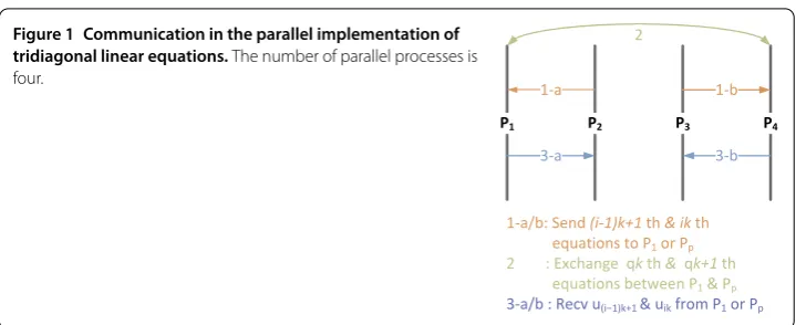
Figure 1 Communication in the parallel implementation of tridiagonal linear equations.The number of parallel processes is four.

We can find the coefficient matrix in equation () is still a tridiagonal matrix. Line  means the reduced system of equations is solved only with processesPandPp.P and Ppdeal with the reduced system of equations using the functions in lines - as well.P

andPpexchange theqkth andqk+ th equations after elimination, and both can obtain u(q+)kandu(q+)k+. In processP,u(i–)k+anduikare acquired and sent toPi( <i≤q). In

processPp,u(i–)k+anduikare got and dispatched toPi(q+ ≤i<p). AfterPi( <i<p)

receivesu(i–)k+ anduikfromPorPp,Uican be solved using equation ().U andUp

can also be figured out by equation () and equation (), respectively.

For the parallel implementation of solving tridiagonal linear equations, there are to-tally three communications shown in Figure . The first communication means thatPi

( <i<p) sends the first and last equations toPorPpafter the elimination. The second

communication indicates thatPandPpexchange theqkth andqk+ th equations in order

to acquireu(q+)kandu(q+)k+simultaneously in the solution of the reduced system. The

third communication is thatPi( <i<p) receivesu(i–)k+anduikfromPorPpafter the

reduced system is solved.

3.3 Implementation

The parallel algorithm for Caputo fractional reaction-diffusion equation with implicit finite-difference method is proposed as shown in Algorithm .F(, ), U(, ), V(),A(, ) are evenly distributed among all processes in order to void the load imbalance. Line  com-putesF(, ),A(),r() and initializesU(, ),V(). Vectorr() is stored in all processes and cal-culated simultaneously. Lines - solve the tridiagonal linear equationsAU_{=Vfor the}

first time. The loop of line  represents iterations on time steps. Since there are depen-dence between the solutions of adjacent time steps, the parallelization of the solution could be carried out only on space steps. In each iteration on time steps, line  solves

Vn₌n–

k=rn––kUk+bn–U+σFn in parallel, and mainly includes parallel

constant-vector multiplications and constant-vector-constant-vector additions. Lines - solve the tridiagonal linear equationsAUn_=Vn_{for the (n+ )th time. As the tridiagonal matrix keeps constant in all}

time iterations, the solution of lines - does not deal with the tridiagonal matrix and only processesVn_{with transform_mid_v() and transform_edg_v(). Particularly, the}

Algorithm :Parallel solution for Caputo fractional reaction-diffusion equation with implicit finite-difference method

input :α,M,N,L,T,f(x,t)

 h←L/M,τ←T/N

 Initiate MPI and getp(MPI Processes Size),Pi(Current Process ID)

 forall MPI processesdo

 Distribute task among MPI processes

 Declare local memory ofF(, ),U(, ),V(),A(, ) in each process

 ComputeF(),A(),r(), and initializeU(, ),V()

 Record timeT

 V()←K∗F(:, )

// solve AU_=V

 ifP_i( <i<p)then

 elimit_down_mid_m(); elimit_up_mid_m(); transform_mid_v()

 else

 elimit_down_edg_m(); elimit_up_edg_m(); transform_edg_v()

 com_form(); solve_reduce(); com_retrieve()

 forn= →Ndo  V()←K∗F(:,n)  forj= →ndo

 V()←V() +U(:,j– )∗r(n–j)

// solve AUn=Vn

 ifPi( <i<p)then

 transform_mid_v()

 else

 transform_edg_v()

 com_form(); solve_reduce(); com_retrieve()

 Record timeT

 OutputT–T

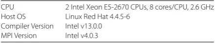
Table 1 The specifications of the experiment’s platform

CPU 2 Intel Xeon E5-2670 CPUs, 8 cores/CPU, 2.6 GHz Host OS Linux Red Hat 4.4.5-6

Compiler Version Intel v13.0.0 MPI Version Intel v4.0.3

4 Experimental results and discussion

The following Caputo fractional reaction-diffusion equation [] is considered, shown in equation ():

⎧ ⎪ ⎨ ⎪ ⎩

Dαtu(x,t) +μu(x,t) = ∂u(x,t)

∂x +Kf(x,t),

u(x, ) = , x∈(, ),

u(,t) =u(,t) = ,

()

withμ= ,K= ,α= ., and

f(x,t) = 

(.)x( –x)t

._{+x( –x)t}_{+ t}_{. ()}

The exact solution of equation () is

u(x,t) =x( –x)t. ()

4.1 Accuracy of parallel solution

For the example in equation (), the parallel solution compares well with the exact ana-lytic solution to the fractional partial differential equation shown in Figure .tandhare

. and

.

. The maximum absolute error is .×

–_{. The difference between serial and}

parallel solution is only .×–_{. When differenttandhare applied, the maximum}

errors between the exact analytic solution and the parallel solution are shown in Table . The maximum error gradually decreases with the increasing number of time and space steps. Altogether, our proposed parallel solution and the exact analytic solution have no noticeable artifacts.

4.2 Performance improvement

The performance comparison between serial solution (SS) and parallel solution (PS) is shown in Table  when differentMandNare applied. In PS,  processes run in parallel. WithM=N= , PS is a little slower than SS. WhenMandNare greater than or equal to , PS is faster than SS. Compared with SS, the speedup of PS increases gradually with

Figure 2 Result comparison between exact analytic solution with parallel solution at time

t= 1.0 andp= 16,M=N= 65.

Table 2 Result comparison between the exact analytic solution and the parallel solution at timet= 1.0 andp= 8, where differentMandNare applied

M = N 65 129 257 513 1,025 2,049

Table 3 Performance comparison between serial solution (SS) and parallel solution (PS) when differentMandNare applied

M = N 65 129 257 513 1,025 2,049

Runtime (s) SS 5.20E–04 3.31E–03 1.22E–02 7.35E–02 4.93E–01 4.03E+00 PS 6.51E–04 1.42E–03 3.75E–03 1.15E–02 4.56E–02 2.77E–01

Speedup 0.80 2.34 3.26 6.37 10.80 14.55

In PS, the number of processes is set to 16.

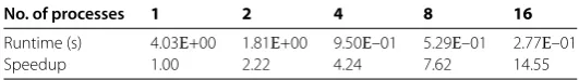
Table 4 Performance of parallel solution withM=N= 2,049 when different numbers of processes are applied

No. of processes 1 2 4 8 16

Runtime (s) 4.03E+00 1.81E+00 9.50E–01 5.29E–01 2.77E–01

Speedup 1.00 2.22 4.24 7.62 14.55

increasingMandN. WhenMandNincrease to ,, the runtime of SS reaches . seconds and that of PS is only .×–seconds. Therefore, the speedup between PS and SS rises to ..

4.3 Scalability

With fixedM=N= ,, the performance comparison among the parallel solutions with a different number of processes is shown in Table . When two parallel processes are used, the speedup is .. When four processes run in parallel, the speedup reaches .. When more than one process is adopted, the total communication cost will increase with the number of parallel processes. However, the speedups in the two situations above outper-form the corresponding perfect speedups. The main reason is that the solution of Caputo fractional reaction-diffusion equation with implicit finite-difference method is memory-intensive, and the decrease of memory overhead by the improvement of data locality is more than the increase of communication cost in the parallelization of two or four pro-cesses. When the number of processes grows to , the speedup is about . times and the scaling efficiency reaches %. Altogether, our proposed parallel solution has good scalability in performance.

5 Conclusions and future work

In this article, we propose a parallel algorithm for time fractional reaction-diffusion equa-tion using the implicit finite-difference method. The algorithm includes a parallel solver for linear tridiagonal equations and parallel vector arithmetic operations. The solver is based on the divide-and-conquer principle and introduces a new tridiagonal reduced sys-tem with an elimination method. The experimental results shows the proposed parallel algorithm is valid and runs much more rapidly than the serial solution. The results also demonstrate the algorithm exhibits good scalability in performance. In addition, the in-troduced tridiagonal reduced system can be regarded as a general method for tridiagonal systems and applied on more applications. In the future, we would like to accelerate the so-lution of time fractional reaction-diffusion equation on heterogeneous architectures [].

Competing interests

Authors’ contributions

Each of the authors contributed to each part of this work equally and read and approved the final version of the manuscript.

Author details

1_{Science and Technology on Parallel and Distributed Processing Laboratory, National University of Defense Technology,}

Changsha, 410073, China. 2_{College of Computer, National University of Defense Technology, Changsha, 410073, China.} 3_{Beijing Satellite Navigation Center, Beijing, 100094, China.}

Acknowledgements

This research work is supported in part by the National Natural Science Foundation of China under Grant Nos. 11175253, 61303265, 61402039, 91430218, 91530324, 61303265, 61170083 and 61373032, in part by Specialized Research Fund for the Doctoral Program of Higher Education under Grant No. 20114307110001, in part by China Postdoctoral Science Foundation under Grant Nos. 2014M562570 and 2015T81127, and in part by 973 Program of China under Grant Nos. 61312701001 and 2014CB430205.

Received: 7 October 2015 Accepted: 28 July 2016

References

1. Podlubny, I: Fractional Differential Equations. Academic Press, San Diego (1999)

2. Debbouche, A, Baleanu, D: Controllability of fractional evolution nonlocal impulsive quasilinear delay integro-differential systems. Comput. Math. Appl.62(3), 1442-1450 (2011)

3. Lenzi, EK, Neto, RM, Tateishi, AA, Lenzi, MK, Ribeiro, HV: Fractional diffusion equations coupled by reaction terms. Phys. A, Stat. Mech. Appl.458, 9-16 (2016)

4. Hristov, J: Approximate solutions to time-fractional models by integral balance approach. In: Fractals and Fractional Dynamics, pp. 78-109 (2015)

5. Bhrawy, AH, Taha, TM, Alzahrani, EO, Baleanu, D, Alzahrani, AA: New operational matrices for solving fractional differential equations on the half-line. PLoS ONE10(5), e0126620 (2015)

6. Doha, EH, Bhrawy, AH, Baleanu, D, Ezz-Eldien, SS: On shifted Jacobi spectral approximations for solving fractional differential equations. Appl. Math. Comput.219(15), 8042-8056 (2013)

7. Ahmad, B, Alhothuali, MS, Alsulami, HH, Kirane, M, Timoshin, S: On a time fractional reaction diffusion equation. Appl. Math. Comput.257, 199-204 (2015)

8. Rida, SZ, El-Sayed, AMA, Arafa, AAM: On the solutions of time-fractional reaction-diffusion equations. Commun. Nonlinear Sci. Numer. Simul.15(12), 3847-3854 (2010). doi:10.1016/j.cnsns.2010.02.007

9. Chen, J, Liu, F, Turner, I, Anh, V: The fundamental and numerical solutions of the Riesz space fractional reaction-dispersion equation. ANZIAM J.50, 45-57 (2008)

10. Chen, J, Liu, F: Stability and convergence of an implicit difference approximation for the space Riesz fractional reaction-dispersion equation. Numer. Math. J. Chin. Univ., Engl. Ser.16(3), 253-264 (2007)

11. Chen, J: An implicit approximation for the Caputo fractional reaction-dispersion equation. J. Xiamen Univ. Natur. Sci.

46(5), 616-619 (2007) (in Chinese)

12. Ding, X-L, Nieto, JJ: Analytical solutions for the multi-term time-space fractional reaction-diffusion equations on an infinite domain. Fract. Calc. Appl. Anal.18(3), 697-716 (2015)

13. Wang, H, Du, N: Fast alternating-direction finite difference methods for three-dimensional space-fractional diffusion equations. J. Comput. Phys.258, 305-318 (2014)

14. Ferrás, LL, Ford, NJ, Morgado, ML, Nóbrega, JM, Rebelo, MS: Fractional Pennes’ bioheat equation: theoretical and numerical studies. Fract. Calc. Appl. Anal.18(4), 1080-1106 (2015)

15. Jiang, Y, Ma, J: High-order finite element methods for time-fractional partial differential equations. J. Comput. Appl. Math.235(11), 3285-3290 (2011)

16. Bhrawy, AH, Abdelkawy, MA, Alzahrani, AA, Baleanu, D, Alzahrani, EO: A Chebyshev-Laguerre-Gauss-Radau collocation scheme for solving a time fractional sub-diffusion equation on a semi-infinite domain. Proc. Rom. Acad., Ser. A16, 490-498 (2015)

17. Bhrawy, AH, Zaky, MA, Baleanu, D, Abdelkawy, MA: A novel spectral approximation for the two-dimensional fractional sub-diffusion problems. Rom. J. Phys.60(3-4), 344-359 (2015)

18. Bhrawy, AH, Doha, EH, Baleanu, D, Ezz-Eldien, SS: A spectral tau algorithm based on Jacobi operational matrix for numerical solution of time fractional diffusion-wave equations. J. Comput. Phys.293, 142-156 (2015)

19. Abdelkawy, MA, Zaky, MA, Bhrawy, AH, Baleanu, D: Numerical simulation of time variable fractional order mobile-immobile advection-dispersion model. Rom. Rep. Phys.67(3), 1-19 (2015)

20. Bhrawy, AH, Zaky, MA, Baleanu, D: New numerical approximations for space-time fractional Burgers’ equations via a Legendre spectral-collocation method. Rom. Rep. Phys.67(2), 1-13 (2015)

21. Rosa, M, Warsa, JS, Perks, M: A cellwise block-Gauss-Seidel iterative method for multigroupSNtransport on a hybrid

parallel computer architecture. Nucl. Sci. Eng.173(3), 209-226 (2013)

22. Gong, C, Liu, J, Chi, L, Huang, H, Fang, J, Gong, Z: GPU accelerated simulations of 3D deterministic particle transport using discrete ordinates method. J. Comput. Phys.230(15), 6010-6022 (2011). doi:10.1016/j.jcp.2011.04.010 23. Wang, Q, Liu, J, Gong, C, Xing, Z: Scalability of 3D deterministic particle transport on the Intel MIC architecture. Nucl.

Sci. Tech.26(5), 50502 (2015)

24. Xu, C, Deng, X, Zhang, L, Fang, J, Wang, G, Jiang, Y, Cao, W, Che, Y, Wang, Y, Wang, Z, Liu, W, Cheng, X: Collaborating CPU and GPU for large-scale high-order CFD simulations with complex grids on the TianHe-1A supercomputer. J. Comput. Phys.278, 275-297 (2014)

25. Wang, Y-X, Zhang, L-L, Liu, W, Che, Y-G, Xu, C-F, Wang, Z-H, Zhuang, Y: Efficient parallel implementation of large scale 3D structured grid CFD applications on the Tianhe-1A supercomputer. Comput. Fluids80, 244-250 (2013) 26. Che, Y, Zhang, L, Xu, C, Wang, Y, Liu, W, Wang, Z: Optimization of a parallel CFD code and its performance evaluation

27. Bai, Z-Z: Parallel multisplitting two-stage iterative methods for large sparse systems of weakly nonlinear equations. Numer. Algorithms15(3-4), 347-372 (1997). doi:10.1023/A:1019110324062

28. Mo, Z, Zhang, A, Cao, X, Liu, Q, Xu, X, An, H, Pei, W, Zhu, S: JASMIN: a parallel software infrastructure for scientific computing. Front. Comput. Sci. China4(4), 480-488 (2010). doi:10.1007/s11704-010-0120-5

29. Yang, B, Lu, K, Gao, Y, Wang, X, Xu, K: GPU acceleration of subgraph isomorphism search in large scale graph. J. Cent. South Univ.22, 2238-2249 (2015)

30. Gong, C, Bao, W, Tang, G, Jiang, Y, Liu, J: Computational challenge of fractional differential equations and the potential solutions: a survey. Math. Probl. Eng.2015, 258265 (2015)

31. Diethelm, K: An efficient parallel algorithm for the numerical solution of fractional differential equations. Fract. Calc. Appl. Anal.14, 475-490 (2011). doi:10.2478/s13540-011-0029-1

32. Gong, C, Bao, W, Tang, G: A parallel algorithm for the Riesz fractional reaction-diffusion equation with explicit finite difference method. Fract. Calc. Appl. Anal.16(3), 654-669 (2013)

33. Gong, C, Bao, W, Tang, G, Yang, B, Liu, J: An efficient parallel solution for Caputo fractional reaction-diffusion equation. J. Supercomput.68(3), 1521-1537 (2014). doi:10.1007/s11227-014-1123-z

34. Chi, L, Liu, J, Li, X: An effective parallel algorithm for tridiagonal linear equations. Chinese J. Comput.22(2), 218-221 (1999) (in Chinese)