R E S E A R C H
Open Access
Very-low-SNR cognitive receiver based on
wavelet preprocessed signal patterns and
neural network
Husam Y. Alzaq
*and B. Berk Ustundag
Abstract
A pattern-based cognitive communication system (PBCCS) that optimizes non-periodic RF waveforms for security applications is proposed. PBCCS is a cross-layer approach that merges the channel encoding and modulation. The transmitter encodes sequences of bits into continuous signal patterns by selecting the proper symbol glossaries. The cognitive receiver preprocesses the received signal by extracting a limited set of wavelet features. The extracted features are fed into an artificial neural network (ANN) to recover the digital data carried by the distorted symbol. The PBCCS system offers a flexible management for robustness against a high noise level and increases the spectral efficiency. In this study, the spectral efficiency and robustness of a PBCCS scheme for an additive white Gaussian noise (AWGN) channel is investigated. The results show that at an SNR of−5 dB, a 3-bit glossary achieves a bit error rate (BER) of 10−5. Also, the link spectral efficiency (LSE) of the proposed system is 2.61 bps/Hz.
Keywords: Cognitive radio (CR), Pattern-based cognitive communication system (PBCCS), Artificial neural network, Wavelet decomposition, Digital signal processing (DSP), Very-low-SNR
1 Introduction
The efficiency of bandwidth utilization takes an impor-tant role in spectrum management [1, 2]. Due to fixed spectrum assignment policies and its inadequate to meet an unexpected increase in the number of higher-data-rate devices, the spectrum is inefficiently used. Cognitive radio (CR) [3–6] was proposed as a promising solution to alleviate the spectrum scarcity problem through dynamic management of the available spectrum. The pioneer work of Mitola et al. [3] led to an efficient utilization of the spec-tral bandwidth by allowing the secondary user (SU), who is not serviced, to detect and access the primary network spectrum gaps. CR allows detection of the state of the spectrum to adjust its own system parameters (transmis-sion power, frequency band, throughput and modulation scheme) in real time [7]. The result is that the utilization of the spectral bandwidth is performed with the soft-ware flexibility in an adaptive manner with respect to the system parameters.
*Correspondence: [email protected]
Department of Computer Engineering, Faculty of Computer Engineering, Istanbul Technical University, Maslak, Ayazaga, 34469 Istanbul, Turkey
However, efficient spectral bandwidth usage under the influence of higher noise is not the major consideration of CR. Claude Shannon [8] showed that the SNR is a lead-ing factor that influences the link spectral efficiency (LSE),
η=C/B, (in bps/Hz). SNR also limits the channel capac-ity. Therefore, the utilization of spectral bandwidth and the robustness to high SNR level are the keys to maximize the channel capacity.
Thus, a pattern-based cognitive communication system (PBCCS) was introduced to optimize the overall spec-tral efficiency with respect to SNR [9, 10]. It is inspired by the recognition capability of humans to concentrate on a single conversation irrespective of the surround-ing loudness. If human ears hear sounds from different sources, the brain chooses to pay attention to a particu-lar voice amongst a whole range of sound streams in an environment. Similar to human cognitive capabilities, the communication system in PBCCS selectively recognizes and recovers the communication signal(s) a into known symbol(s), even within the same frequency range.
1.1 Related work
Conventional cognitive radio is equipped with various techniques for making wireless systems more flexible and robust to channel variation. Mitola, in his disserta-tion [11], stated that, although many aspects of wireless networks are artificial, they may still be enhanced by machine learning (ML). Recently, machine learning algo-rithms have become one of the key enabling features of cognitive radio in many applications. In previous litera-ture, many techniques and algorithms have been applied to the cognitive radio engine [12, 13], such as the artificial neural network (ANN), hidden Markov model (HMM), fuzzy logic control, meta-heuristic algorithms (evolution-ary/genetic algorithm) and rule-based systems [14–16].
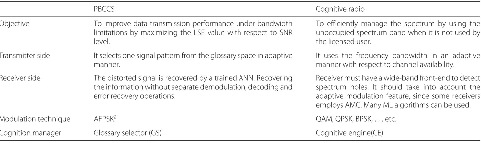
On the other hand, the PBCCS structure is an extension for CR, which is a cross-layer architecture. The control unit of PBCCS is located in the data-link layer and com-municates with the external glossary space that manages the transmission process. Table 1 summarizes the sim-ilarities and differences between PBCCS and cognitive radio.
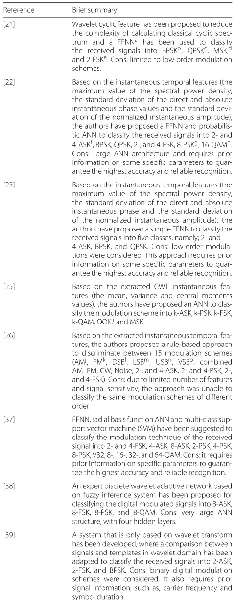
Generally, ANN has been adapted in the cognitive radio engine for various modulation classification, known as automatic modulation recognition (AMR) or automatic modulation classification (AMC). For instance, ANN was implemented for channel sensing [17–19] and spectrum prediction [17, 20], etc. To enhance ANN classification accuracy, ANN is usually combined with the extracted fea-tures from the received signal, which allows the engine to have the capability to identify the modulation scheme at low SNR levels. Cyclic spectral analysis [17], wavelet cyclic features [21], temporal feature-based modulation [22, 23], carrier frequency and baud rate [24], and contin-uous wavelet transform (CWT) [25] are some examples of these features. Dahap et al. [26] proposed a digital recog-nition algorithm that uses six features extracted from instantaneous information and signal spectrum to dis-criminate between different modulated signals. Table 2 shows a brief summary of these approaches. However,
most of the aforementioned approaches have been used to classify low-order modulation technique, such as 2-ASK and 2-PSK. In addition, a prior signal information such as the carrier frequency is required. Additionally, if these approaches classify high-order modulation schemes, they construct a large ANN. The PBCCS is a kind of AMC that has not only the ability to classify high-order modula-tion, but also can encode the received analog signal at very low SNR.
In this work, we choose to use the ANN model at the PBCCS receiver owing to its powerful capabilities. ANN can predict the correct class of the received signal even if the input signals have not been seen before, which allow the model to learn from training dataset and generalize the model to any received signal. Moreover, ANN is a non-linear model and hence can predict the nonnon-linear received signal better than the linear model. Finally, the ANN par-allel processing and the appropriate simple structure are two important properties for realizing ANN on hardware. Furthermore, we have implemented a cognitive radio solution, which offers flexibility between the available spectrum and SNR. This solution has the capability to bal-ance between LSE and the overall channel capacity under a very low SNR. It constructs optimal communication symbols, which compensate for the difference in data rates under various noise levels. In addition, the PBCCS system integrates the modulator and channel encoder through a cross-layer approach. The binary data is encoded into the appropriate waveform according to the selected glossary. Each binary word is assigned to the artificially constructed patterns. The transmitter selects the appropriate set of patterns that maximize LSE.
1.2 Contribution
In our previous work [27], we have experimentally inves-tigated the performance of PBCCS in an additive white Gaussian noise (AWGN) channel by employing 2-level Daubechies-2 wavelet (DB2) as a discrete wavelet trans-formation (DWT) to preprocess the received signal. With
Table 1Comparison between pattern based cognitive communication system and cognitive radio
PBCCS Cognitive radio
Objective To improve data transmission performance under bandwidth limitations by maximizing the LSE value with respect to SNR level.
To efficiently manage the spectrum by using the unoccupied spectrum band when it is not used by the licensed user.
Transmitter side It selects one signal pattern from the glossary space in adaptive manner.
It uses the frequency bandwidth in an adaptive manner with respect to channel availability.
Receiver side The distorted signal is recovered by a trained ANN. Recovering the information without separate demodulation, decoding and error recovery operations.
Receiver must have a wide-band front-end to detect spectrum holes. It should take into account the adaptive modulation feature, since some receivers employs AMC. Many ML algorithms can be used.
Modulation technique AFPSKa QAM, QPSK, BPSK,. . .etc.
Cognition manager Glossary selector (GS) Cognitive engine(CE)
Table 2ANN within cognitive radio
Reference Brief summary
[21] Wavelet cyclic feature has been proposed to reduce the complexity of calculating classical cyclic spec-trum and a FFNNa has been used to classify the received signals into BPSKb, QPSKc, MSK,d and 2-FSKe. Cons: limited to low-order modulation schemes.
[22] Based on the instantaneous temporal features (the maximum value of the spectral power density, the standard deviation of the direct and absolute instantaneous phase values and the standard devi-ation of the normalized instantaneous amplitude), the authors have proposed a FFNN and probabilis-tic ANN to classify the received signals into 2- and 4-ASKf, BPSK, QPSK, 2-, and 4-FSK, 8-PSKg, 16-QAMh. Cons: Large ANN architecture and requires prior information on some specific parameters to guar-antee the highest accuracy and reliable recognition.
[23] Based on the instantaneous temporal features (the maximum value of the spectral power density, the standard deviation of the direct and absolute instantaneous phase and the standard deviation of the normalized instantaneous amplitude), the authors have proposed a simple FFNN to classify the received signals into five classes, namely; 2- and 4-ASK, BPSK, and QPSK. Cons: low-order modula-tions were considered. This approach requires prior information on some specific parameters to guar-antee the highest accuracy and reliable recognition.
[25] Based on the extracted CWT instantaneous fea-tures (the mean, variance and central moments values), the authors have proposed an ANN to clas-sify the modulation scheme into k-ASK, k-PSK, k-FSK, k-QAM, OOK,iand MSK.
[26] Based on the extracted instantaneous temporal fea-tures, the authors proposed a rule-based approach to discriminate between 15 modulation schemes (AMj, FMk, DSBl, LSBm, USBn, VSBo, combined AM–FM, CW, Noise, 2-, and 4-ASK, 2- and 4-PSK, 2-, and 4-FSK). Cons: due to limited number of features and signal sensitivity, the approach was unable to classify the same modulation schemes of different order.
[37] FFNN, radial basis function ANN and multi-class sup-port vector machine (SVM) have been suggested to classify the modulation technique of the received signal into 2- and 4-FSK, 4-ASK, 8-ASK, 2-PSK, 4-PSK, 8-PSK, V32, 8-, 16-, 32-, and 64-QAM. Cons: it requires prior information on specific parameters to guaran-tee the highest accuracy and reliable recognition.
[38] An expert discrete wavelet adaptive network based on fuzzy inference system has been proposed for classifying the digital modulated signals into 8-ASK, 8-FSK, 8-PSK, and 8-QAM. Cons: very large ANN structure, with four hidden layers.
[39] A system that is only based on wavelet transform has been developed, where a comparison between signals and templates in wavelet domain has been adapted to classify the received signals into 2-ASK, 2-FSK, and BPSK. Cons: binary digital modulation schemes were considered. It also requires prior signal information, such as, carrier frequency and symbol duration.
Table 2ANN within cognitive radio (Continued)
[40] A system that is based solely on DWT and sig-nals statistics was used to classify the modulated received signals into 16-QAM, QPSK and BPSK. Cons: degradation of performance at SNR appeared when the ANN was trained on signals with lower SNR.
aFFNN: Feed-forward neural network bBPSK: Binary phase shift keying cQPSK: Quadrature phase shift keying dMSK: Minimum shift keying ek-FSK:k−bit Frequency shift keying fk-ASK:k−bit Amplitude shift keying gk-PSK:k−bit Phase shift keying
hk-QAM:k−bit Quadrature amplitude modulation iOOK: On-off keying
jAM: Amplitude modulation kFM: Frequency modulation lDSB: Double sideband modulation mLSB: Lower sideband modulation nUSB: Upper sideband modulation oVSB: Vestigial sideband
regards to this, in the current work, learning the appro-priate communication patterns for the cognitive receiver and the influence factors on the received symbols are being studied. The main contributions of this paper are in fourfold.
• We analyzed various DWT approaches, which have an influence on the recognition rate of the ANN. • We studied the effect of using 4- and 5-level DWT,
which reduce the size of the ANN.
• We analyzed various back-propagation learning algorithms, which have an influence on system performance as well as the speed of learning. • Finally, we showed that the space complexity of the
receiver exhibits a reduced ANN structure in terms of inputs and the hidden layer. As fewer resources were used, the receiver could be implemented with fewer hardware units.
1.3 Paper organization
The rest of this paper is organized in the following way. Section 2 describes the structure of the PBCCS model and its blocks in detail. It also gives a short introduction on wavelet and neural networks. In Section 3, we evaluate the performance of the PBCCS system. In Section 4, we conclude the paper and recommend directions for future work.
2 PBCCS structure
2.1 The transmitter of PBCCS
The transmitter of PBCCS is responsible for three tasks: 1) selecting the appropriate glossary with respect to the SNR level, 2) encoding the user data, and 3) transmitting the signal through the antenna. In PBCCS, the modula-tion is performed by using the sinusoidal pattern envelope construction (SPEC) algorithm [10]. The SPEC algorithm is used to prevent unwanted extra spectral usage, and it guarantees that the signal’s pattern ends at its initial point to ensure a zero-power density in average and has no high-frequency components.
The SPEC algorithm has two essential parame-ters—namely, “depth”, and “level”. Depth determines the length of the pattern in terms of the time—i.e., number of periods. Meanwhile, level identifies a value for each feature of the signal pattern. It represents the maximum and the minimum values of any signal characteristics (amplitude (A), frequency (F) or phase (P) at depthi. All possible outcomes in the SPEC algorithm are due to the changes in the A, F, and P features of the signal.
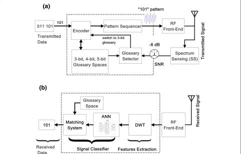
Figure 1a shows the block diagram of the transmitter, which consists of an encoder, a glossary space, and a glos-sary selector. The glosglos-sary is an information encoding method. It is composed of different patterns generated by
the SPEC algorithm. The SPEC is responsible for com-bining different sinusoidal waveforms to form a symbol as shown in Eq. (1). The generated signal of each symbol has different waveforms that change over time in terms of amplitude, frequency, and phase.
mi(t)= J
i=0
ai∗xi(t)∗cos
2∗π∗fi∗t+φi
(1)
wheremi(t)is theithpattern;ai,fiandφiare the
ampli-tude, frequency and phase of the signal, respectively;Jis the total number of sinusoidal waves that the pattern con-tains (determined by the depth parameter); and xi(t) is
defined as
xi(t)=
1 if 2∗π∗i≤t<2π∗(i+1)+2π,
0 otherwise (2)
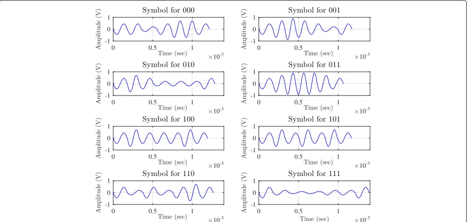
Each block of k input data bits di,i = 1, 2,. . ., 2k is
mapped to patternmi(t). All symbols,mi(t), are combined
to form a k-bit glossary space. Figure 2 illustrates a 3-bit glossary space, containing eight signal patterns. In this work, the performance of 3-bit, 4-bit, and 5-bit glossary spaces, with 8, 16, and 32 patterns, respectively, is studied.
(a)
(b)
Fig. 2The 3-bit glossary space with 5 levels, each of which has 7 patterns (depth is set to 6). The signal’s amplitude is [ 0.1, 0.2, 0.45, 0.7, 0.9] V, frequency is [ 4.600, 5.000, 5.600, 6.600, 7.400] kHz, and phase shift is [−π/2−π/4 0π/4π/2] rad
The transmitted symbol,m(t), contains a sequence of known data symbols, m1(t),m2(t), .... According to the selected glossary, the pattern that matches the data index is selected and applied to the RF front-end.
The glossary selector is the core component in the trans-mitter’s design, because it selects the most appropriate glossary from the glossary space as part of the adapta-tion process. It takes the glossary space informaadapta-tion and channel spectral situation—i.e., the SNR value from the environment, as an input to determine the most proper glossaries set in the glossary space by computing the max-imum likelihood value. For example, Fig. 1 shows that the measured SNR is -8 dB. Therefore, the glossary selector switches to a 3-bit glossary and maps ‘101’ to the sixth pattern (shown in Fig. 2).
2.2 The receiver of PBCCS
The main modules of the receiver are the discrete wavelet transform unit and ANN, as illustrated in Fig. 1b. The aim of using ANN at the receiver is to predict the original bits of the distorted received signal. The receiver does not con-struct a similar analog signal or estimate its parameter. Instead, it classifies the input samples to a known pattern, so that the correct bits can be inferred. In the following subsections, we briefly describe the functionality of each part of the receiver.
2.2.1 Features extraction and reduction
One of the aspects of signal classification is the selec-tion of proper classificaselec-tion features. The goal of
fea-ture extraction is to obtain a set of feafea-tures that can discriminate different received signals. In this work, the discrete wavelet transform (DWT) [28] is used to extract the signal features.
The discrete wavelet transform is a linear signal pro-cessing technique that transforms a signal r(t) from the time domain to the “wavelet” domain—i.e., wavelet coef-ficients. A transformation from the time domain to the “wavelet” domain is analogous to the Fourier transform. The key difference between wavelet transform and Fourier transform is that wavelets are local in both time (via translation) and frequency (via dilation), whereas Fourier analysis is local only in frequency but not in time. Because the generated waveforms contain numerous nonstation-ary or transitory characteristics, which are often the most important parts of signals, Fourier analysis is unsuitable to describe such characteristics. Moreover, the received pat-tern signal can be represented by a compact form and hold most features that distinguish it from other patterns. As a result, the wavelet analysis is appropriate to capture the changes in the pattern’s frequency over time and achieves better lossy compression, which dramatically reduces the size of ANN.
In general, the received signal,r(t), can be modeled in the AWGN channel as follows:
r(t)=ms(t)+wn(t) (3)
wherems(t)denotes the original pattern signal, andwn(t)
discretized in time so thatn−point discrete signalr[n] is constructed. The DWT is defined by Eq. (4) as follows:
W(j,k)=
j
k
r(k)ψjk(n), j,k∈Z (4)
ψjk(n)=2−j/2ψ
2−jn−k (5)
where W(j,k) are the wavelet transform coefficients;
ψjk(n) is the mother wavelet, andj andk are the scale
parameter and shift parameter, respectively. In practice, it is inconvenient to apply Eq. (4) in calculating the coefficients. The DWT can be implemented as a series of high-pass and low-pass filters, called the recursive wavelet transform, which decomposes the signalx[n] into two parts. The wavelet decomposition depends mainly on orthonormal filter banks. Figure 3 shows the signal decomposition by a two-channel wavelet structure, where x[n] is the input signal,h[n] is the high-pass filter,g[n] is the low-pass filter, and↓ 2 is the down-sampling by a factor of two. In this way, each filter creates a series of coefficients that represent and compact the original information of the signal.
Mathematically, a signalx[n] is composed of high and low frequencies as shown in Eq. (6). It shows that the obtained signal can be represented by using half the coef-ficients because they are decimated by 2.
x[k]=xhigh[k−1]+xlow[k−1] (6)
The filtered and decimated output of low-pass part is recursively passed through identical wavelet filter banks to add the dimension of varying resolution at every stage. Equations (7) and (8) are mathematical expressions of filtering a signal through a digital high-pass filter h[n] ,
and low-pass filter g[n]. This operation corresponds to convolution with an impulse response ofk−tap filters.
yhigh[k]=
n
x[n] .h[2k−n] (7)
ylow[k]=
n
x[n] .g[2k−n] (8)
wherenbecomes 2nrepresenting the down-sampling pro-cess. The output of the low-pass filter, ylow[k], provides
approximation signal, whereas the output of the high-pass filter,yhigh[k], provides detailed signal. In addition, Eqs. (7) and (8) show that using DWT can not only greatly reduce the number of input nodes, but also effectively expresses the features of the received signal, thereby enhancing the ability of neural networks to recognize the signal.
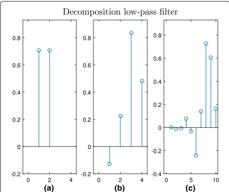
A variety of different wavelet families has been pro-posed in the literature. In this work, the simplest wavelet family—i.e., the Haar wavelet and triangle wavelet are selected [28]. In addition, the 4- and 10-coefficient wavelet family (the second and the fifth orders of Daubechies wavelet—i.e., DB2, DB5), and the 6-coefficient wavelet family coiflets (C6) proposed by Daubechies are used [29]. The decomposition low-pass filter parameters of the Haar, DB2 and DB5 wavelet are shown in Fig. 4.
2.2.2 Recognition layer
After extracting the proper features from the received sig-nal, classifying these patterns into appropriate classes is the final step to recognize the symbol. In this work, the artificial neural network (ANN) [30, 31] is considered as a recognition layer to recover the transmitted data, and it forms the cognitive part of the PBCCS receiver.
The main reason for choosing the preprocessed wavelet with ANN is its high sensitivity for recognizing the ampli-tude, frequency and phase changes in the communica-tion signal. The output that is produced by the ANN is
(a) (b) (c)
Fig. 4Low-pass filter parameters of different wavelet families.aHaar, bDB2,cDB5
decoded in the final stage into the correct bit sequence, as shown in Fig. 5.
In this work, the most common ANN model, namely multilayer perceptron (MLP), is used. MLP is a type of feed-forward neural network (FFNN) model that maps the input data onto a set of appropriate outputs. It con-sists of at least three layers—i.e., the input layer, one or more hidden layers and an output layer. The network is fully connected from one layer to the next as a directed acyclic graph (Fig. 5). Each neuron is capable of multi-plying the inputs by its weight and sum up the results. In other words, the neuron operations are performed by multipliers and adders.
Mathematically, fornarbitrary distinct received samples
(xi,ti), wherexi is the extracted features’ vector from the
received signal,xi =[xi1,xi2,. . .,xin]T∈ Rnandti is the
target vector,ti = [ti1,ti2,. . .,tim]T ∈ Rm. nandmare
the size of the input feature and the target vectors, respec-tively. The target vectortirepresents the actual sequence
of bits that the recognition layer must produce.
A single hidden layer of a FFNN (Fig. 5) with an activa-tion funcactiva-tion,g(.)andkhidden neurons is mathematically modeled as
g n
i=1
wji·xi+bj
=yj, j=1, 2,. . .,k (9)
wherewji =
wj1,wj2,. . .,wjk T is the weight vector
con-necting thejthhidden neurons with the inputs and bj is
the bias value of thejthhidden neuron. The bias allows the sigmoid function curve to be shifted horizontally along the input axis while leaving the shape of the function unchanged.wji·xidenotes the inner product ofwjiandxj.
The result of thejthoutput neuron can be mathemati-cally computed as shown in Eq. (10):
g ⎛ ⎝k
i=1
βji·yi+bj
⎞
⎠=Oj, j=1, 2,. . .,M (10)
where Mis the total number of output neurons. βji =
βj1,βj2,. . .,βjm T is the weight vector connecting thejth
hidden neurons and output neurons and bj is the bias
value of thejthoutput neuron.
Because the final goal is to find the relation between the inputxi and the targetti, the activation functiong(.)
can approximate thesenreceived samples with zero mean
Fig. 5Feed-forward ANN (FFNN) with one hidden layer and an output layer. The extracted features are fed into ANN withninput nodes, andkand
error, such that N
The back-propagation algorithm (BP) [30] is used to compute the weights and biases of the ANN by mini-mizing the error function in weight space using gradient descent.
The received sequence of bits, aˆ = ˆa1,aˆ2,. . .,aˆm
is approximated from the output neurons as shown in Eq. (12):
whereOjis thejththe output neuron.
As a final point, the structure of the FFNN should be modular and simple, so that the hardware architecture can be efficiently realized on floating point digital signal pro-cessor (DSP) or a field programmable gate array (FPGA). As there are various combinations of designing a FFNN, an efficient design should include the following aspects
• Input neurons: the number of neurons is equivalent to the sample size of the DWT vector.
• Hidden neurons: due to low complexity and high applicability perspective [10], a single hidden layer with few number of neurons should be used. The number of neurons will be determined by the cross validation method.
• Output neurons: The number of output neurons should be identical to the size of the glossary space—i.e., total number of patterns. However, each glossary differs in the number of symbols that it represents. For instance, the3−bit glossary has8 symbols while4−bit glossary has16symbols. Therefore, the size of the glossary can be added to determine the width of the output sequence bits.
3 Experimental results
In this section, the performance of the proposed PBCCS based on the extracted features (discussed in Section 2) is verified in an AWGN channel. At the end of this section, the proposed approach complexity is presented.
3.1 Simulation settings
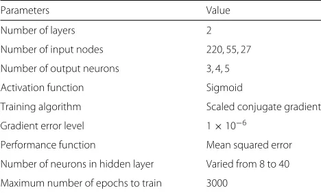
Simulations were carried out to transmit 2kdifferent sym-bols (k-bit glossary) at various SNR levels. The SNR levels were in the range of [−15, 25] dB. The ANN parameters are shown in Table 4. All experiments were performed using Matlab software.
3.2 Constructing the glossary
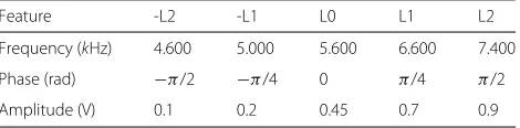
Each test pattern is constructed with five sub-signal. According to the SPEC algorithm, patterns are generated with bandwidth-limited switching among different fre-quency, phase, and amplitude levels. The features of the communication signal (frequency, phase, and amplitude) are chosen from five different levels, listed in Table 3. The depth is set to 6, which indicates that each signal symbol is constructed from 7 sub-patterns.
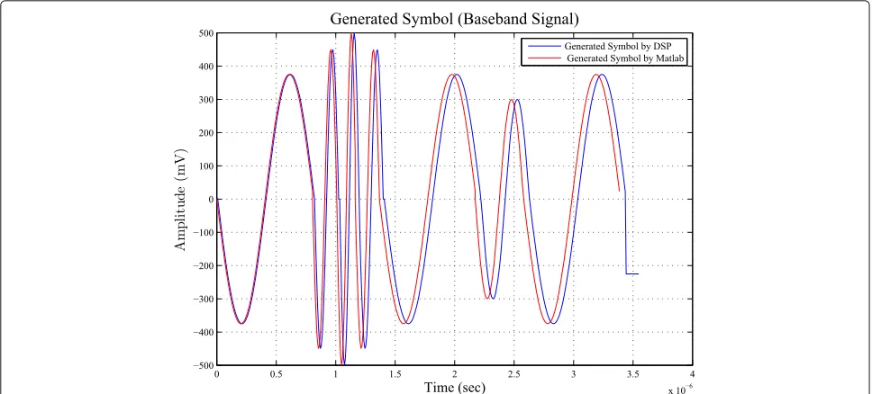
Synthetic signals that represent the symbols was vali-dated on hardware. For this purpose, we used an FMC150 [32] daughter card attached to a Xilinx ML605 board [33]. The FMC150 is a dual 14-bit channel ADC and dual channel 16-bit DAC FMC daughter card. Figure 6 shows the synthesized signal by the hardware against a sim-ulated signal generated by Matlab. There are 7 sub-patterns in each signal. The frequencies of each pattern are 1.25, 5, 6.25, 5, 1.25, 2.5, and 1.25 MHz. The ampli-tude and phase are identical to the values presented in Table 3. The frequency of the simulated signal might slightly differ from the real one owing to the register preci-sion of the FMC150—i.e., the measured frequency of each sub-pattern is 1.229, 4.9020, 6.1728, 4.9020, 1.229, 2.457, and 1.229 MHz. The mean voltage of the baseband signal is 2.9710∗10−4, which is approximately zero.
3.3 Learning process and model evaluation
Before assessing the system, two datasets were generated for each symbol. These sets should be used for learning (training) and testing (evaluating). The learning set is used to derive the model offline, whereas the test set is used to estimate model’s accuracy online, as shown in Fig. 7. Symbols that were used during the learning stage would not be involved in the testing stage. Moreover, the learn-ing dataset should be larger than the testlearn-ing dataset, so that the model can be built from a large space of sampled signals. For example, the dataset of the 3-bit glossary con-tains 248, 000 symbols and 74, 400 symbols for learning and testing, respectively. In other words, 70% of the total symbols were used for learning.
To assess the accuracy of the wavelet filter banks and ANN model, we use the success rate of the recognition symbol as an indication of the effectiveness of the receiver to correctly recognize the received symbols. It indicates the capability of the trained model to classify the received symbols in the testing set, which were not seen before.
Table 3Base signal specifications
Feature -L2 -L1 L0 L1 L2
Frequency (kHz) 4.600 5.000 5.600 6.600 7.400
Phase (rad) −π/2 −π/4 0 π/4 π/2
Fig. 6Synthetic signal (baseband signal) by using Matlab compared with the real synthetic signal generated by the hardware.Fs=122.88 MHz
It also expresses the probability of correct classification, which is computed as follows:
Success Rate= 1
N
N
i xi∗100 (13)
where N is the total number of test symbols and xi is
an indicator whose value is 1 if the ith symbol is cor-rectly received. In other words,Success Ratemeasures the symbol error rate (SER).
In addition to the success rate, the BER performance is used to assess the accuracy of the whole system. It expresses the number of bit errors per second divided by the total number of transferred bits.
3.4 Classification performance of different wavelet families
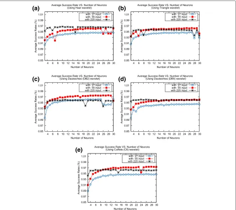
In this section, we study the effect of applying differ-ent wavelet families on the performance of the receiver for 3-bit glossary. The received signal has 880 samples. The number of input nodes was subsequently reduced from 220 to 55 and 27 to identify the most relevant input features to ANN by employing 2-, 4-, and 5-level DWT decomposition (j=2, 4 and 5). The ANN model was then trained for different numbers of neurons in the hidden
layer. These experiments were repeated 10 times, and the success rate was averaged.
Figure 8a illustrates the effect of using the Haar wavelet for various numbers of neurons in the input and hidden layers. It shows that the average success rate of the model is more than 90% for all scenarios. By using 27 neurons at the input layer, the success rate is greater than 94% with 12 neurons or more at the hidden layer.
In Fig. 8b, the effect of using a triangle wavelet is shown, which is similar to Fig. 8a. However, the success rate of the model with 55 neurons outperforms the model that has 220 inputs. The improvement of the input size reduction to 55 inputs by using DB2 is illustrated in Fig. 8c. The suc-cess rate is greater than 97% with more than 12 hidden neurons (with the exception of the case with 27 inputs).
DB5 wavelet has similar performance compared to the DB2, as shown in Fig. 8d. Similar result was also obtained by using a coiflets (C6) wavelet as shown in Fig. 8e. The figure shows that with 55 input nodes and 10 hidden nodes, the performance is improved compared with the experiment of 220 input nodes.
To analyze the previous results, the success rates of PBCCS are elaborated in the [−20, 15] dB range for var-ious network configurations in the hidden layer (Fig. 9).
When the SNR is equal to or greater than−12 dB, the
(a)
(b)
(c)
(e)
(d)
Fig. 8The probability of correct classification (average success rate) vs. number of hidden neurons by using different wavelet transforms and various input size in an AWGN channel.aHaar wavelet,bTriangle wavelet,cDaubechies (DB2) wavelet,dDaubechies (DB5) wavelet,eCoiflets (C6) wavelet
(a)
(b)
success rate is greater than 99.0% for all configurations, which means that there is no error in the received sym-bols (SER= 0.1). Below−12 dB, the success rate linearly decreases to 65%. In all cases, using 10 hidden neurons or more layer does not improve the success rate.
In summary, we found that for 3-bit glossary the DB2 wavelet has better performance compared with other wavelet families studied in our tests. It is also found that
with a 27−input ANN, the performance is better than
that when using many extracted features. Furthermore, the use of 14 hidden neurons or more has a similar recog-nition rate to a network that contains 8 hidden neurons. As a result, an ANN that is based on 5-level DWT can be realized with 27 inputs and as minimum as 14 hidden neu-rons. This reduction will use fewer resources during the hardware design realization.
3.5 Classification performance of various learning algorithms
In this section, we examined four popular back-propagation learning algorithms—namely, (Levenberg-Marquardt (LM), scaled conjugate gradient (SCG), gradient descent with momentum and adaptive learning rate back-propagation (GDX) and Bayesian regularization back-propagation (BR) in terms of speed and the num-ber of iterations to achieve the same performance goal (MSE)=0.01. The ANN parameters are set according to Table 4. For LM algorithm, the maximum number of iter-ations was set to 25 to limit the learning time as shown in Table 5. It is worth mentioning that we choose the best parameters for LM algorithms by experimental study.
The average training accuracies of each algorithms over various ANN structures are shown in Fig. 10a. It indi-cates that all learning algorithms achieve 96%. The LM algorithm is failed in some experiments because the algorithm reaches the maximum number of iterations (Fig. 10b). Figure 10c shows that as the number of hid-den units increases, the learning time of both LM and BR algorithms is significantly increased, whereas the learning
Table 4ANN parameters
Parameters Value
Number of layers 2
Number of input nodes 220, 55, 27
Number of output neurons 3, 4, 5
Activation function Sigmoid
Training algorithm Scaled conjugate gradient
Gradient error level 1×10⁻⁶
Performance function Mean squared error
Number of neurons in hidden layer Varied from 8 to 40
Maximum number of epochs to train 3000
Table 5ANN parameters
Parameter Value
Maximum number of epochs to train 25
Initialμvalue 0.1
Decrease factor (α) 0.2
Increase factor (β) 6
Minimum performance gradient 10−5
Performance function Mean squared error
time of both SCG and GDX algorithms is constant and less than 20 m. The average learning time of BR and LM with 40 hidden units network are 3 and 2 h, while the number of iterations is less than 25 and 100 iterations, which means that both algorithms have high computation complexity.
The average MSE versus number of hidden neurons are shown in Fig. 10d. Smaller values that are close to zero are better because they indicate that the MLP had fitted the data well. SCG, GDX, and BR learning algorithms have better performance compared with LM algorithm because the number of iterations of LM was limited to 25 itera-tions. Increasing the number iterations will improve the MSE values but has dramatically effect on learning time.
3.6 System performance withk-bit glossary spaces in AWGN Channel
Based on the previous results, DB2 wavelet decomposition was applied to extract 27 features from the received signal. We simulated the BER by applying 3∗105at each SNR level and measuring the number of uncorrected received bits. In Fig. 11, the SNR curves illustrate the 3-, 4-, and 5-bit glossary performance with various hidden neurons. The total area under each curve indicates the overall system performance under different noise and data bit error rate (BER) levels. It means that the carve with minimum area has a better performance. It is depicted in Fig. 11a that the BER is 10−5at−5 dB for most ANN configurations. Sim-ilarly, Fig. 11b presents that the curve for 20 neurons has SNR of approximately−2 dB at 10−5. Also, it shows that the system performance improves with increasing number of neurons due to the fact that the recognition capability could be enhanced as the number of hidden neurons is increased. Figure 11c shows similar performance as shown in Fig. 11b except that SNR is approximately 4 dB at 10−5. Figure 11 shows a strange behavior as the BER carve reaches 10−5, where some errors increases again. We expect that the ANN could not distinguish between the samples either because the learning process is not enough or it overfits the data.
(a)
(b)
(c)
(d)
Fig. 10Comparison between SCG, LM, GDX and BR learning algorithms with respect toaAverage success rate (accuracy).bAverage number of iterations.cAverage Learning time.dAverage MSE performance
neurons is approximately equal to an ANN configuration with higher hidden units. This phenomenon indicates that an increasing number of hidden neurons does not always improve the performance. As a result, the best PBCCS performance can be realized with a fixed-structure ANN of 27 inputs nodes and 20 hidden neurons for 3-, 4-, and 5-bit glossaries.
3.7 Spectral efficiency
The ability of the system to balance between the spec-tral efficiency under a very low SNR is an advantage of the proposed scheme. For each glossary, we construct
a random signal of 2000 symbols to measure the aver-age data rate and the occupied bandwidth. Table 6 shows the spectral efficiency, η, of the previous constructed glossaries.
The most significant feature of the proposed method is its competence to operate in a region beyond the Shannon boundary. The Shannon boundary is drawn in Fig. 12 by using the Shannon limit theorem (equation(6.5—49), [2]), which is rewritten as follows:
Eb
N0 > 2η−1
η (14)
(a)
(b)
(c)
Table 6Spectral efficiency of PBCCS atPe=10−5bit error
probability
Glossary 3-bit 4-bit 5-bit
M (symbols) 8 16 32
SNR value (dB) -5 -2 4
Data rate (kbps) 2.508 3.553 4.6
Average BW (kHz) 0.960 0.881 0.9135
LSE,η, (bps/Hz) 2.61 4.0318 5.03
where,
η <log2
1+ EbR N0W
=log2
1+ηEb N0
(15)
Equation 14 states the condition of reliable communi-cation in terms of bandwidth efficiency, η, and power efficiency in terms ofEb/N0. Figure 12 shows the
mini-mum value ofEb/N0 = −1.59 for which reliable com-munication is possible. The marks in the figure show the best working point regarding the glossary at a 10−5 bit error rate andM−QAM. This figure depicts that the 4-bit glossary and 16-QAM have the same spectral efficiency, but the 4-bit glossary is more robust to high levels of AWGN than 16-QAM. Similarly, 5-bit glossary is more
robust than 32−QAM at the same spectral efficiency,
η=5.
However, the most interesting finding is that the 3−bit glossary breaks down the Shannon limits. This phe-nomenon occurs because the ANN can perfectly discrim-inate among the eight signals of the 3−bit glossary. In the learning step, the ANN model has constructed a model
Fig. 12Comparison between PBCCS andm-QAM in an AWGN channel atPe=10−5bit error probability. The neural network contains 20 hidden neurons
that allows the PBCCS to classify any unseen signal, in a manner analogous to memory. Another reason for break-ing down the Shannon limit is the usage of non-periodic signals. Shannon’s law is restricted to periodic signals [34]. The PBCCS constructs a non-periodic and uncorrelated communication waveforms that provide a manageable SNR capability between high noise redundancy and high data bandwidth requirements under observed spectrum conditions.
It is worth mentioning that this result depends on the difference between the bandwidth of recovered digital data based on a priori information in the glossary and the raw physical data bandwidth inside the communica-tion medium. In addicommunica-tion, the synchronizacommunica-tion overhead between the transmitted symbols is not considered.
3.8 Bit error rate comparison
A comparative analysis between the PBCCS and of the matched filter is shown in Fig. 13. The total area under each curve indicates the overall system perfor-mance under different noise and data BER levels. Accord-ing to Fig. 13, 3−, 4−, 5-bit glossary constructed by PBCCS modulation have 20 dB, 21 dB and 22 dB better
performances at 10−5 BER than 8-QAM, 16-QAM, and
32-QAM, respectively. It is worth noting that eachk-bit symbol space has 2ksymbols asm-QAM becausem=2k. Also, 3−, 4−, 5-bit glossary outperforms the 4−, 8−, 16-PSK by 16, 17, and 23 dB.
The bit error probability for 16-QAM is given by decreasing function of its argument; the probability of error decreases as the ratio4Eb
5No increases. This means that
the decision boundary of the QAM technique depends on increasing the signal energy, which makes the binary signals dissimilar. However, the PBCSS depends not only on the signal energy but also on the extracted features from the received signal by DWT and the nonlinear model of ANN, which enable the PBCCS model to reduce the probability of error.
3.9 System performance comparison with AMC
Because this work and similar works have used different methodologies in signal type recognition, direct compar-ison with these works is difficult. Table 7 compares the PBCCS with some of AMC techniques. A brief summary of each recognition approach was given in Table 2. It is clear that the proposed PBCCS outperforms the previous approaches (at -11 dB) because the symbols that are stored
in the glossary was designed with properties that allow the ANN to discriminate between them.
3.10 Receiver space complexity
After simulating the proposed approach, the next step is to verify the design on real hardware such as a field-programmable gate array (FPGA) and application-specific integrated circuit (ASIC). We prefer using FPGA because the parallel structure of an ANN and the similarity of neurons makes its design simple and straightforward.
Each FPGA comes with limited resources, which poses challenges for real implementation. Space complexity gives an indication of the number of used functional units. It approximates the numbers of connections, multipliers and adders that the real design will occupy when it is implemented on an FPGA.
The transmitter could be implemented by means of memory. Each glossary requires one memory (blocked RAM (BRAM)), which is indexed by the transmitted bits. For example, Xilinx Virtex VI xc6vlx240t-1ff1156 has 416 BRAMs, each storing 36 Kb [33]. Figure 14 shows the block diagram of the PBCCS transmitter, where the preamble was used for the synchronization. It shows only 3-bit glossary with 13×16 BRAM.
At the receiver, each neuron of the implemented ANN has a set of multipliers that are used to multiply the
Table 7Comparison between different works in terms of features, ANN model and the achieved SNR with the recognition accuracy
Reference Application Applied features Type of ANN Recognition accuracy (%)
[22] AMC Instantaneous temporal
feature-based
FANN (5,19,8) and PANN (5,1800,8)
Overall success rate at -5 db are 65.63% and 55.5% respectively.
[23] AMC Instantaneous temporal
feature-based modulation
FANN (4,7,5) the overall success rate at -5 dB is 99.65%.
[25] AMC Continuous wavelet
transform (CWT)
N/A The overall success rate at 0 dB
is 99.6% (using 10 features).
[26] AMC Instantaneous information
and signal spectrum
N/A The overall success rate at 3 dB
is 98.6% (using 10 features).
[37] AMC Combination of the higher
order moments, higher
The overall success rate at -3 dB is 87.50%. The overall success rate at -3 dB is 86.45%.
[38] AMC 7-level DWT Adaptive Network Based
Fuzzy Inference Systems of 5 hidden layers
The overall success rate using DB2 at -5 dB is 98%.
[39] AMC Haar Wavelet Transform N/A The overall success rate at -7 dB
is 99.71%.
[40] AMC Haar Wavelet Transform N/A The overall success rate at 5 dB
is 97.93%.
[27] Modulation classification and signal encoding
1-level DB2 DWT FFNN(30,14,3) The overall success rate a -11 dB for 3-bit glossaries is 96.0%.
PBCCS Modulation classification and signal encoding
5-level DB2 DWT FFNN(27,14,3), FFNN(27,14,4), FFNN(27,14,5)
Fig. 14The block diagram of the PBCCS transmitter
weight of the connections with the received data val-ues. For example, if there are 26 2-input nodes, then each hidden neuron requires 26 multipliers and 26 2-input adders (including one adder to the bias). Because multipliers are more expensive than the adders and each FPGA comes with a limited number of them, they, in fact, significantly influence the design. For instance, Xilinx Virtex VI xc6vlx240t-1ff1156 has 768 multipliers (named DSP48E1) [33].
Table 8 shows a comparison between the architecture of the proposed approach compared with the one that is based on time delay ANN (TDNN) [10]. It shows that the total number of multipliers in the FFNN is drastically reduced compared with the TDNN. Moreover, the 3-bit glossary space requires 26∗20∗3 = 1560 connections. This indicates the number of internal connections among the input, hidden and output layers of any used neural
network, whereas TDNN requires 120∗20∗3 = 7200
connections.
In addition to the impact of the neural network, the wavelet decomposition has effect on the space complexity
Table 8Space complexity comparison between the proposed approach and time delay ANN [10]
Parameters Wavelet and ANN Time delay ANN
k=3 k=4 k=3 k=4
Number of layers 2 2 2 2
bit size of glossary space 3 4 3 4
Input neurons 27 27 120 120
Hidden neurons 20 20 20 50
Output neurons 3 4 3 4
Number of multipliers 600 620 2460 2480
of the receiver. Similar to the finite impulse response (FIR) filter, the wavelet decomposition convolves wavelet coefficients with the received signals. This convolution process requires as many multiplication resources as the number of filter taps. For example, DB2 and DB5 can be implemented as 4-tap and 10-tap FIR filters, respectively. Furthermore, it is an iterative process—i.e., the output of one stage is an input to the next stage (Fig. 3). The direct implementation DWT, known as the multiply-accumulate structure (MAC), requires as many resources as the number of stages times the numbers of filter taps—i.e., 5-level DB2 requires 20 multipliers. An alternative but efficient implementation could be achieved by means of the distributed arithmetic algorithm (DAA) [35, 36]. DAA efficiently realizes the sum-of-products computation by means of memory (LUT), adders and shift registers, with-out employing any multipliers. That is, the total number of multipliers at the receiver will not be affected by the DWT implementation.
4 Conclusions
PBCCS was designed to increase the spectral efficiency by constructing a secure and non-periodic communica-tion signals. In addicommunica-tion, PBCCS minimizes the bit error rate through optimized signal patterns that are decoded solely by DWT preprocessed signals and artificial neural network.
appropriate operating point of the glossary selector with the discrete wavelet family at the receiver. We found out that the DB2 wavelet decomposition filter shows better performance compared with the other studied wavelet families. Thanks to DWT, a simple ANN structure was constructed with few hidden neurons, which is impossi-ble for a third-party to predict. In addition, we studied the effect of various back-propagation learning algorithm. We could conclude that in terms of learning time and per-formance, both SCG and GDX are better to handle large dataset that includes thousands of signals. Finally, because of robustness to stationary noise, the proposed approach has a great advantage of less bit error, unlike the standard modulation techniques, which has higher bit error rate.
The simulation results also reveal that by using 5-level DWT and a neural network, SNR values of -5 dB, -2 and 4 dB are achieved at a BER of 10−5for 3-bit, 4-bit and 5-bit glossary spaces, respectively. The advantage is obvious, because the transmitter can adapt the bit rate accord-ing to SNR values. Therefore, adaptive glossary and its performance can be considered in a future work.
An initial evaluation of hardware implementation was demonstrated, and the applicability of the proposed mod-ulation technique and the recognition layer were dis-cussed. In brief, according to our preliminary works on the FPGA platform, the system can be realized with limited level glossaries in the existing technology. The next future step of this work is validating the simulation and prelimi-nary laboratory testbed results under real application and environmental conditions.
Acknowledgements
The authors would like to thank the anonymous reviewers for their valuable comments and suggestions to improve the quality of the article.
Funding
There are no sources of funding body reported for this manuscript.
Authors’ contributions
All authors contributed to the work. All authors read and approved the final manuscript.
Competing interests
The authors declare that they have no competing interests.
Publisher’s Note
Springer Nature remains neutral with regard to jurisdictional claims in published maps and institutional affiliations.
Received: 24 January 2017 Accepted: 12 June 2017
References
1. DM Dobkin,RF Engineering for Wireless Networks: Hardware, Antennas, and Propagation (Communications Engineering). (Newnes, USA, 2004) 2. JG Proakis, M Salehi,Digital Communication, 5th edn. (McGraw-Hill
Education, New York, 2008)
3. J Mitola, JGQ Maguire, Cognitive radio: making software radios more personal. Pers. Commun. IEEE.6(4), 13–18 (1999). doi:10.1109/98.788210
4. S Haykin, Cognitive radio: brain-empowered wireless communications. Selected Areas Commun. IEEE J.23(2), 201–220 (2005). doi:10.1109/JSAC. 2004.839380
5. S Haykin,Cognitive Dynamic Systems: Perception-action Cycle, Radar and Radio. (Cambridge University Press, New York, 2012)
6. T Yucek, H Arslan, A survey of spectrum sensing algorithms for cognitive radio applications. Commun. Surv. Tutorials IEEE.11(1), 116–130 (2009). doi:10.1109/SURV.2009.090109
7. IF Akyildiz, W-Y Lee, MC Vuran, S Mohanty, NeXt generation/dynamic spectrum access/cognitive radio wireless networks: a survey. Intl. J. Comput. Telecommun. Netw.50(13), 2127–2159 (2006). doi:10.1016/j.comnet.2006.05.001
8. CE Shannon, A mathematical theory of communication. Bell Syst. Technical J.27(3), 379–423 (1948). doi:10.1002/j.1538-7305.1948. tb01338.x
9. B Ustundag, O Orcay, inCognitive Radio Oriented Wireless Networks and Communications, 2008. CrownCom 2008. 3rd International Conference On. Pattern Based Encoding for Cognitive Communication, (2008), pp. 1–6. doi:10.1109/CROWNCOM.2008.4562494
10. B Ustundag, O Orcay, A pattern construction scheme for neural network-based cognitive communication. Entropy.13(1), 64–81 (2011). doi:10.3390/e13010064
11. J Mitola,Cognitive Radio: An Integrated Agent Architecture for Software Defined Radio. Doctor of technology. (Royal Institute Technology (KTH), Stockholm, 2000)
12. N Ahad, J Qadir, N Ahsan, Neural networks in wireless networks: techniques, applications and guidelines. J. Netw. Comput. Appl.68, 1–27 (2016). doi:10.1016/j.jnca.2016.04.006
13. N Abbas, Y Nasser, KE Ahmad, Recent advances on artificial intelligence and learning techniques in cognitive radio networks. EURASIP J. Wirel. Commun. Netw.2015(1), 174 (2015). doi:10.1186/s13638-015-0381-7 14. A He, KK Bae, TR Newman, J Gaeddert, K Kim, R Menon, L Morales-Tirado,
JJ Neel, Y Zhao, JH Reed, WH Tranter, A survey of artificial intelligence for cognitive radios. Veh. Technol. IEEE Trans.59(4), 1578–1592 (2010). doi:10.1109/TVT.2010.2043968
15. M Alshawaqfeh, X Wang, AR Ekti, MZ Shakir, K Qaraqe, E Serpedin, in
Cognitive Radio Oriented Wireless Networks: 10th International Conference, CROWNCOM 2015, Doha, Qatar, April 21-23. Revised Selected Papers, ed. by M Weichold, M Hamdi, ZM Shakir, M Abdallah, KG Karagiannidis, and M Ismail. A Survey of Machine Learning Algorithms and their Applications in Cognitive Radio (Springer, Cham, 2015), pp. 790–801
16. M Bkassiny, Y Li, SK Jayaweera, A survey on machine-learning techniques in cognitive radios. IEEE Commun. Surv. Tutorials.15(3), 1136–1159 (2013). doi:10.1109/SURV.2012.100412.00017
17. A Fehske, J Gaeddert, J Reed, inNew Frontiers in Dynamic Spectrum Access Networks, 2005. DySPAN 2005. 2005 First IEEE International Symposium On. A new Approach to Signal Classification Using Spectral Correlation and Neural Networks, (2005), pp. 144–150. doi:10.1109/DYSPAN.2005.1542629 18. S Baban, D Denkoviski, O Holland, L Gavrilovska, H Aghvami, inPersonal
Indoor and Mobile Radio Communications (PIMRC), 2013 IEEE 24th International Symposium On. Radio Access Technology Classification for Cognitive Radio Networks, (2013), pp. 2718–2722. doi:10.1109/PIMRC. 2013.6666608
19. S Baban, O Holland, H Aghvami, inWireless Communication Systems (ISWCS 2013), Proceedings of the Tenth International Symposium On. Wireless Standard Classification in Cognitive Radio Networks Using Self-Organizing Maps, (Ilmenau, 2013), pp. 1–5
20. X Xing, T Jing, W Cheng, Y Huo, X Cheng, Spectrum prediction in cognitive radio networks. Wirel. Commun. IEEE.20(2), 90–96 (2013). doi:10.1109/MWC.2013.6507399
21. L Zhou, H Man, inVehicular Technology Conference (VTC Fall), 2013 IEEE 78th. Wavelet Cyclic Feature Based Automatic Modulation Recognition Using Nonuniform Compressive Samples, (2013), pp. 1–6.
doi:10.1109/VTCFall.2013.6692456
22. MMT Abdelreheem, MO Helmi, inTelecommunications (BIHTEL), 2012 IX International Symposium On. Digital Modulation Classification through Time and Frequency Domain Features using Neural Networks, (2012), pp. 1–5. doi:10.1109/BIHTEL.2012.6412073
24. A Attar, A Sheikhi, A Zamani, inTelecommunications and Networking - ICT 2004. Lecture Notes in Computer Science, ed. by J de Souza, P Dini, and P Lorenz. Communication System Recognition by Modulation Recognition, vol. 3124 (Springer, Berlin Heidelberg, 2004), pp. 106–113
25. M Walenczykowska, A Kawalec, Type of modulation identification using wavelet transform and neural network. J. Pol. Acad. Sci.64(1), 257–261 (2016). doi:10.1515/bpasts-2016-0028
26. BI Dahap, L HongShu, M Ramadan, inThe Proceedings of the Second International Conference on Communications, Signal Processing, and Systems. Lecture Notes in Electrical Engineering, ed. by B Zhang, J Mu, W Wang, Q Liang, and Y Pi. Simple and Efficient Algorithm for Automatic Modulation Recognition for Analogue and Digital Signals, vol. 246 (Springer, Switzerland, 2014), pp. 345–357
27. H Alzaq, BB Ustundag, inEuropean Wireless 2015; 21th European Wireless Conference, Proceedings Of. Wavelet Preprocessed Neural Network Based Receiver for Low SNR Communication System, (Budapest, 2015), pp. 1–6 28. S Mallat,A Wavelet, Tour of Signal Processing, The Sparse Way, 3rd edn.
(Academic Press, Philadelphia, 2008)
29. I Daubechies,Ten Lectures on Wavelets. Society for Industrial and Applied Mathematics, (Philadelphia, 1992)
30. S Haykin,Neural Networks and Learning Machines, 3rd edn. (Prentice-Hall, Inc., Upper Saddle River, 2008)
31. YF Hassan, Rough sets for adapting wavelet neural networks as a new classifier system. Appl. Intell.35(2), 260–268 (2011). doi:10.1007/s10489-010-0218-3
32. 4DSP, Design and system integration for digital signal processing. 4DSP -FMC150. Available at http://www.4dsp.com/-FMC150.php/
33. Xilinx Inc., Virtex-6 FPGA ML605 Evaluation Kit. Available at http://www. xilinx.com/products/boards-and-kits/ek-v6-ml605-g.html
34. J Prothero,The Shannon Law for non-periodic channels. Technical Report R-2012-1. (Astrapi Corporation, Washington, D.C., 2012)
35. A Peled, B Liu, A new hardware realization of digital filters. Acoust. Speech Signal Process. IEEE Trans.22(6), 456–462 (1974). doi:10.1109/TASSP.1974. 1162619
36. SA White, Applications of distributed arithmetic to digital signal processing: a tutorial review. ASSP Mag. IEEE.6(3), 4–19 (1989). doi:10.1109/53.29648
37. A Ebrahimzadeh, R Ghazalian, Blind digital modulation classification in software radio using the optimized classifier and feature subset selection. Eng. Appl. Artif. Intell.24(1), 50–59 (2011). doi:10.1016/j.engappai.2010. 08.008
38. E Avci, D Hanbay, A Varol, An expert discrete wavelet adaptive network based fuzzy inference system for digital modulation recognition. Expert Syst. Appl.33(3), 582–589 (2007). doi:10.1016/j.eswa.2006.06.001 39. S Hassanpour, AM Pezeshk, F Behnia, in2015 38th International Conference
on Telecommunications and Signal Processing (TSP). A Robust Algorithm Based on Wavelet Transform for Recognition of Binary Digital Modulations, (2015), pp. 508–512. doi:10.1109/DASC.2012.6382368 40. D Digdarsini, M Kumar, G Khot, T Ram, V Tank, in2014 International