Variable coefficient KdV equation with time dependent variable coefficient topographic forcing term and atmospheric blocking

R E S E A R C H

Open Access

Variable coefficient KdV equation with

time-dependent variable coefficient

topographic forcing term and atmospheric

blocking

Juanjuan Ji

_{, Lanfang Zhang}

_{, Longxue Wang}

_{, Shengping Wu}

_{and Lihua Zhang}

*_{Correspondence:[email protected]} 1_{School of Physics and Electrical}

Engineering, Anqing Normal University, Anqing, China Full list of author information is available at the end of the article

Abstract

This paper mainly focuses on solitary waves excited by topography with

time-dependent variable coefficient. By making use of multiple scale expansion and multiple level approximation method, a variable coefficient KdV equation with variable coefficient topographic forcing term is derived from barotropic and potential vorticity equation on a beta-plane including topography effect. In the derivation, removingy-average trick, a higher order term of stream function including five arbitrary functions and forced topography is introduced. Taking the strict solution of the standard constant coefficient KdV equation as the initial value, the approximate analytical solution of the derived equation is obtained by means of homotopy analysis method. Based on the new equation and its analytical solution, some complicated and changeable atmospheric blocking phenomena might be explained when some functions are selected appropriately.

PACS Codes: 02.30.Jr; 05.45.Yv

Keywords: Atmospheric blocking; Time-dependent variable coefficient topographic forcing term; Higher order term including forcing topography; Approximate analytical solution

1 Introduction

Atmospheric blocking is an important large-scale weather phenomenon. When atmo-spheric blocking occurs at mid-high latitudes, it often causes extraordinary flood, ex-treme drought or exex-treme cold, and other abnormal phenomena. Usually an atmospheric blocking anticyclone has three types of patterns: monopole-type blocking, dipole-type blocking, and multi-pole type blocking. In the past decades, a large number of constant-coefficient nonlinear equations have been derived, for example, the famous Korteweg de Vries (KdV), modified KdV (mKdV), nonlinear Schrödinger (NLS) equations, and so on. However, analytical solutions of these deduced constant coefficient equations are impos-sible to describe the formation, development, and extinction of the complicated atmo-spheric blocking life cycle. The nonlinear variable coefficient equations can be used to explain atmospheric blocking phenomena. Ref. [1] used the derived variable coefficient KdV system to explain well the life cycle of a blocking system. In fact, blocking phenomena

are related to beta effect, energy dispersion, topography, and other forcing factors. Yang and Chen [2–4] derived Boussinesq-BO equation, generalized Boussinesq equation, and generalized inhomogeneous KdV-Burgers equation considering dissipation effect and to-pography. The topography plays very important roles in atmospheric blocking evolution. A series of research works about topography forcing effect have been carried out [5–8], most of which still involved constant coefficient nonlinear equations.

In this paper, combining variable coefficient thought with the effect of topographic forc-ing, starting from barotropic and potential vorticity equation on a beta-plane including topographic effect, a variable coefficient KdV equation with time-dependent variable co-efficient forced term is derived.

At present, there are many analytical methods [9–15] for solving nonlinear partial differ-ential equations, for example,q-homotopy analysis transform method [16–18], homotopy analysis method [19,20], homotopy perturbation method [21], and so on. However, solv-ing analytical solutions of variable coefficient equation with forced term is a long-standsolv-ing difficulty. Consider the KdV equation with forced term in Ref. [22]

UT+a(T)UUX+b(T)U2UX+c(T)UXXX+d(T)UX+γ(T)U=Γ(T), (1)

where the analytical solutions were obtained, and the interaction of multiple wave solu-tions was presented. In Ref. [23], the new exact solitary wave solution and periodic wave solution of Eq. (2) KdV-Burgers equation with forcing term were obtained.

ut+αuux+βuxx+γuxxx=f(t). (2)

Obviously, forcing terms of Eqs. (1)–(2) are all functions of time. But research into exact analytical solutions of KdV type equation with forced term about variablexorXis almost blank. The homotopy analysis method (HAM) [24] is very powerful, we select it to solve the approximate analytic solution of the derived equation in this paper.

The main purpose of this paper is to derive a new variable coefficient KdV equation with forced term and investigate the evolution process of atmospheric blocking. The structure of this paper is as follows. A new model is derived from a non-dimensional barotropic and potential vorticity equation on a beta-plane including topography effect in Sect.2. In Sect.3, an approximate analytic solution of the derived equation is obtained by HAM, and the evolution process of stream function field is investigated in different parameters. In Sect.4, discussion is presented. Finally, our conclusions are given.

2 Derivation of variable-coefficient KdV equation with time-dependent variable coefficient topographic forcing term

In barotropic atmosphere, the known barotropic and potential vorticity equation includ-ing topography effect on a beta-plane can be written in the form [25]

∂ ∂t

∇2_{ψ–Fψ+Jψ,∇}2_ψ+h+β∂ψ

∂x = 0, (3)

whereψ=ψ(x,y,t) is a non-dimensional stream function,∇2₌ ∂2 ∂x2+

∂2

∂y2 is the horizontal

Laplace operator,J(a,b) = ∂a_∂x∂b_∂y–∂a_∂y∂b_∂x is the Jacobian ofaandb,β= (L2_/U)β

(2ω0/a0)cosϕ0,ω0is the angular frequency of the earth’s rotation,a0is the radius of the

earth, ϕ0 is the latitude,F= (L/R0)2,U andLare the characteristic horizontal velocity

and the characteristic horizontal length, respectively,R0is the Rossby deformation radius,

h=h(x,y) is non-dimensional topography height distribution.

In order to consider weakly nonlinear perturbations on a zonal flow, we introduce a small parameterε1, then assume

ψ(x,y,t) =Ψ0(y,t) +εψ(x,y,t), (4)

where the basic flowΨ0(y,t) is a function abouty,t,ψ(x,y,t) is a perturbation stream

function.

Substituting Eq. (4) into Eq. (3) and omittingofψ(x,y,t), we obtain the following equa-tion for perturbaequa-tion stream funcequa-tion:

∂

We adopt the following transform:

X=ε12_{(x–c0t), T=ε}32_{t, h(x,y) =ε}2_{H(X,y). (6)}

Suppose topography can be separated as

Equation (9) can be further simplified as follows:

The asymptotic expansion is imported for a perturbation stream functionψin the form

ψ=ψ0+εψ1+ε2ψ2+· · ·. (11)

Taking the substitution of Eq. (11) into Eq. (10) and requiring all the coefficients of dif-ferent powers ofεto be zero yield

ε0: (c0+Ψ0y)

We suppose that Eq. (12) has the following variable separation solution:

ψ0=G0(y,T)A(X,T). (14)

whereF1(y) is an arbitrary integration function abouty,F1yis the first order differential

toy.

In order to derive an arbitrary variable coefficient KdV equation with forced term, we introduce the following higher order termψ1with forced term:

Therefore, whenBi(i= 1, 2, 3, 4, 5) satisfy the following equations:

(c0+Ψ0y)2(FΨ0yy+F1yy) –Ψ0yy(c0+Ψ0y)(c0F+FΨ0y+F1y+β)G20

– 2(c0+Ψ0y)3B1yy+ 2(c0+Ψ0y)2(c0F

+FΨ0y+F1y+β)B1–a1G0(c0+Ψ0y)(F1y+β) = 0, (24)

(c0+Ψ0y)2G0+ (c0+Ψ0y)2B2yy– (c0+Ψ0y)(c0F+FΨ0y+F1y+β)B2

+a2G0(F1y+β) = 0, (25)

Ψ0yT(F1y+β) + (c0+Ψ0y)3B4yy– (c0+Ψ0y)2(c0F+FΨ0y+F1y+β)B4

+a3G0(F1y+β) = 0, (26)

Ψ0y(c0+Ψ0y) + (c0+Ψ0y)2B5yy– (c0+Ψ0y)(c0F+FΨ0y+F1y+β)B5

–a4G0(F1y+β) = 0, (27)

whereB3is an arbitrary function, we can obtain a new variable coefficient KdV equation with forcing term

∂A

∂t +a1A

∂A

∂X+a2

∂3A

∂X3+a3A=a4

∂H1

∂X . (28)

In Eqs. (24)–(28),ai=ai(T) (i= 1, 2, 3, 4) are arbitrary functions aboutT. Obviously,

forcing term of Eq. (28) contains time-dependent variable coefficient a4(T) and topo-graphic forcing term ∂H1

∂X. Consequently, Eq. (28) is called variable coefficient KdV

equa-tion with time-dependent variable coefficient topographic forcing term.

3 Approximate analytic solution of derived equation and complicated atmospheric blocking phenomena

In this section, we first solve approximate analytical solution of Eq. (28) by HAM in Ref. [24]. Equation (28) can be rewritten as

LA(X,T) +PA(X,T) +BA(X,T) = 0, (29)

where L= ∂

∂T is a linear operator, LA(X,T) = ∂A

∂T, P is an auxiliary linear operator,

PA(X,T) =a2_∂X∂3A3 +a3A,Bis a nonlinear operator,BA(X,T) = a1

2

∂A2 ∂X –a4

∂H ∂X.

Taking variable coefficients as

a1=c1sin(T), a2=c2,

a3=c3cos(T), a4=c4,

(30)

wherec1,c2,c3,c4are arbitrary constants, we take forced topography as

H(X) =n0cos(mX), (31)

We make use of the strict solution of the standard constant coefficient KdV equation in the solitary theory as initial value, namely

A0(X,T) = 2k2sech2(kX), (32)

whereis an auxiliary parameter.

Whenm> 1, we obtain the following equations:

+ 2c4mn0sin(mX)T– 0.5T2c2c42m4n0cos(mX)

+c3c42mn0sin(mX)cos(T) +c3c42mn0sin(mX)sin(T)T. (37) Then the second-order HAM approximate analytical solution of Eq. (28) is as follows:

A(X,T) =A0(X,T) +A1(X,T) +A2(X,T). (38) When the basic flowΨ0(y,t) is taken to be

Ψ0=b0y+b1, (39)

whereb0,b1are arbitrary constants, and using Eqs. (15)–(16), we obtain

G0(y,T) =R(T)sin obtain the first-order approximate solution of the original equation Eq. (3) in the form

–c0t) 2c1cosε32_{t–c1–c1cos}2_ε32_{t+ 12c2sinε}32_t

– 12c2cosε32_tε32_{t– 16k}5_{c2tanh(kX)sech}2_k√_ε(x

–c0t) 2ε32_t–c3sinε32_t+Tc42_mn0sinm√_ε(x–c0t)

–c3c42mn0sinm√ε(x–c0t)+ 2c4mn0sinm√ε

·(x–c0t)

ε32_{t– 0.5T}2_c

2c42m4n0cos

m√ε(x–c0t)

+c3c42mn0sin

m√ε(x–c0t)

cosε32_t

+c3c42mn0sinm√ε(x–c0t)sinε32_tε32_{t, (41)}

whereR(ε32t) is an arbitrary function aboutt.

When takingR(ε32t) in the form

Rε32_t=k1sech20ε32_{(t– 9), (42)}

other parameters are as follows:

F= 1.5, c0= –2.4, c1= 2.7, c2= 5.3, c3= 1.3, c4= 0.6,

β= 16.3, b0= –18,

b1= 5, n0= 5.2, m= 1.4, ε= 0.1, k= 6, k1= 10.

(43)

The evolution of stream function field is shown in Fig.1. When

a1=c1sinε3/2t, a2=c2, a3=c3cosε3/2t,

a4=c4eε3/2t, R=k1sech 30ε32_{(t– 4),}

(44)

where c1,c2,c3, c4 are arbitrary constants, andc4= 9.6, β= 16.3,b0= –8,b1= 5,n0=

5.2,m= 2.8,ε= 0.05,k1= 20, other parameters are the same as those for Fig.1,Ψ0,G0

are shown in Eqs. (39)–(40), solving process is similar to above, no longer repeated, the evolution of stream function field is shown in Fig.2.

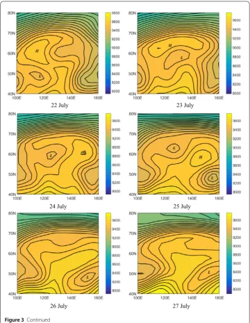
In order to enhance the practical significance of our work, we take a real observational blocking case that happened during 14 July 2003 to 27 July 2003 as a simple example. Making use of the National Centers for Environmental Prediction–National Center for Atmospheric Research (NCEP-NCAR) reanalysis data, a dipole blocking event is depicted in Fig.3.

4 Discussions

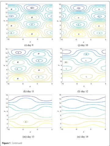
Figure 1Whena1=c1sin(ε3/2t),a2=c2,a3=c3cos(ε3/2t),a4=c4, the evolution of stream function field, the

stream function analytic expression is Eq. (43), whereR=k1sech[20ε 3

2_{(t– 9)],F= 1.5,c0= –2.4,c1= 2.7,}

Figure 1Continued

then become weaker, finally disappearing after the fourth day (Fig.1(h)). We still call it dipole blocking, and its life-time is fourteen days.

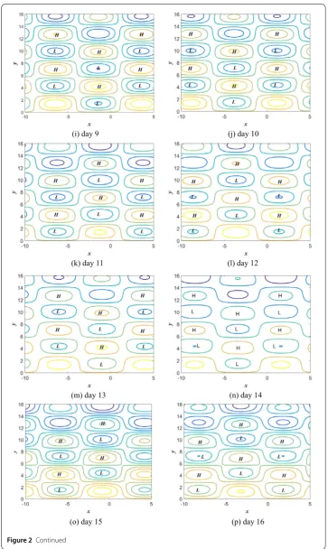
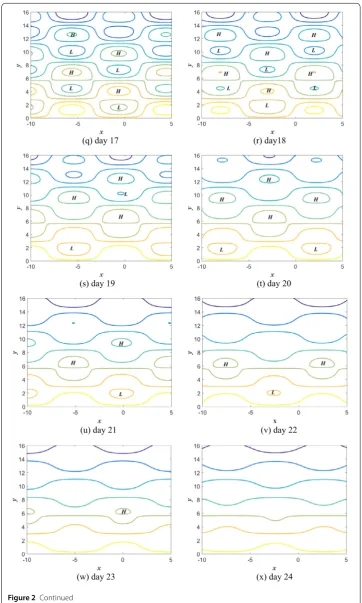
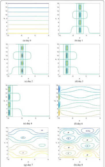
Figure2reveals a complicated dipole blocking process. At the initial time, a weak dipole is presented (Fig.2(a)). From the second to sixth day, stream function field presents multi-pole status (Fig.2(b)–(f )); on the seventh day, multi-dipoles appear (Fig.2(g)), on the four-teenth day, multi-dipoles disappear (Fig.2(n)), then a dipole appears (Fig.2(o)). After the twenty-fourth day, the dipole disappears (Fig.2(x)). Obviously, stream function field pos-sesses a process from dipole to multi-pole then to multi-dipole, again to dipole, finally disappearing, but we still call it dipole blocking, and its life-time is twenty-four days.

Figure 2Whena1=c1sin(ε3/2t),a2=c2,a3=c3cos(ε3/2t),a4=c4eε 3/2_t

, the evolution of stream function field,R=k1sech[20ε3/2(t– 9)],F= 1.5,c0= –2.4,c1= 2.7,c2= 5.3,c3= 1.3,c4= 9.6,β= 16.3,b0= –8,b1= 5,

Figure 3Continued

of dipole (16–27 July 2003). We still call it dipole blocking. Besides, from 16 July 2003 to 27 July 2003, the dipole gradually moves westward.

Figure1and Fig.2reveal the complexity of dipole blocking evolution. However, Fig.2

5 Conclusions

In this paper, combining topographic forcing effect with time-varying property and in-troducing a higher order term of the stream function with five arbitrary functions and forced topography, a variable coefficient KdV equation with time-dependent variable co-efficient topographic forcing term is obtained. When selecting some proper parameters, stream function field presents a complicated and changeable dipole-type blocking. Conse-quently, time-dependent variable coefficient and forced topography have great influence on the evolution of stream function field. With appropriate selection of arbitrary functions and constants, many kinds of real atmospheric phenomena may be successfully explained.

Funding

The work was supported by the National Natural Science Foundation of China (No. 51607004), Natural Science Research Project of Education Department of Anhui Province (No. KJ2019A0566, No. KJ2018A0369).

Declaration

This manuscript is a small part of both funds No. 51607004, No. KJ2019A0566 and No. KJ2018A03699.

Competing interests

The authors declare that they have no competing interests.

Authors’ contributions

The authors declare that the study was realized in collaboration with the same responsibility. All authors read and approved the final manuscript.

Author details

1_{School of Physics and Electrical Engineering, Anqing Normal University, Anqing, China.}2_{Anqing meteorological bureau,}

Anqing, China.

Publisher’s Note

Springer Nature remains neutral with regard to jurisdictional claims in published maps and institutional affiliations.

Received: 8 August 2018 Accepted: 26 February 2019

References

1. Tang, X., Huang, F., Lou, S.: Variable coefficient KdV equation and the analytical diagnoses of a dipole blocking life cycle. Chin. Phys. Lett.23, 887–890 (2006)

2. Yang, H., Yang, D., Shi, Y., et al.: Interaction of algebraic Rossby solitary waves with topography and atmospheric blocking. Dyn. Atmos. Ocean.71, 21–34 (2015)

3. Yang, H.W., Yin, B.S., et al.: Forced solitary Rossby waves under the influence of slowly varying topography with time. Chin. Phys. B20, 120203 (2011)

4. Chen, Y.D., Yang, H.W., Gao, Y.F., et al.: A new model for algebraic Rossby solitary waves in rotation fluid and its solution. Chin. Phys. B24, 54–61 (2015)

5. Yang, H.W., Yin, B.S., Shi, Y.L.: Forced dissipative Boussinesq equation for solitary waves excited by unstable topography. Nonlinear Dyn.70, 1389–1396 (2012)

6. Yang, H.W., Yin, B.S., et al.: Forced solitary Rossby waves under the influence of slowly varying topography with time. Chin. Phys. B20, 120203 (2011)

7. Song, J., Yang, L.G., Liu, Q.S.: Solitary Rossby waves with beta effect and topography effect in a barotropic atmospheric model. Prog. Geophys.27, 393–397 (2012)

8. Giannitsis, C., Lindzen, R.S.: Nonlinear saturation of topographically forced Rossby waves in a Barotropic model. J. Atmos. Sci.58, 2927–2941 (2001)

9. Yang, X.J., Gao, F., Srivastava, H.M.: A new computational approach for solving nonlinear local fractional PDEs. J. Comput. Appl. Math.339, 285–296 (2018)

10. Yang, X.J., Gao, F., Srivastava, H.M.: Exact travelling wave solutions for the local fractional two-dimensional Burgers-type equations. Comput. Math. Appl.73, 203–210 (2016)

11. Yang, X.J., Machado, J.A.T., Baleanu, D.: Exact traveling-wave solution for local fractional Boussinesq equation in fractal domain. Fractals25, 1740006 (2017)

12. Yang, X.J., Gao, F., Machado, J.A.T., et al.: Exact travelling wave solutions for local fractional partial differential equations in mathematical physics. In: Mathematical Methods in Engineering, pp. 175–191. Springer, Cham (2019)

13. Yang, X.J., Tenreiro Machado, J.A., Baleanu, D., et al.: On exact traveling-wave solutions for local fractional Korteweg–de Vries equation. Chaos, Interdiscip. J. Nonlinear Sci.26, 110–118 (2016)

14. Yang, X.J., Gao, F., Srivastava, H.M.: Exact travelling wave solutions for the local fractional two-dimensional Burgers-type equations. Comput. Math. Appl.73, 203–210 (2017)

16. Saad, K.M.: Comparing the Caputo, Caputo–Fabrizio and Atangana–Baleanu derivative with fractional order: fractional cubic isothermal auto-catalytic chemical system. Eur. Phys. J. Plus133, 94 (2018)

17. Saad, K.M., Baleanu, D., Atangana, A.: New fractional derivatives applied to the Korteweg–de Vries and Korteweg–de Vries–Burger’s equations. Comput. Appl. Math.37, 5203–5216 (2018)

18. Saad, K.M., Abdon, A., Dumitru, B.: New fractional derivatives with non-singular kernel applied to the Burgers equation. Chaos, Interdiscip. J. Nonlinear Sci.28, 063109 (2018)

19. Jafarian, A., Ghaderi, P., Golmankhaneh, A.K., Baleanu, D.: Analytical approximate solutions of the Zakharov–Kuznetsov equations. Rom. Rep. Phys.66, 296–306 (2014)

20. Jafarian, A., Ghaderi, P., Golmankhaneh, A.K., Baleanu, D.: Analytical treatment of system of Abel integral equations by homotopy analysis method. Rom. Rep. Phys.66, 603–611 (2014)

21. Golmankhaneh, A.K.: Solving of the fractional non-linear and linear Schrodinger equations by homotopy perturbation method. Rom. Rep. Phys.54, 823–832 (2009)

22. Liu, Y., Gao, Y.T., Sun, Z.Y., et al.: Multi-soliton solutions of the forced variable-coefficient extended Korteweg–de Vries equation arisen in fluid dynamics of internal solitary waves. Nonlinear Dyn.66, 575–587 (2011)

23. Abazari, R.: Application of extended Tanh method on KdV–Burgers equation with forcing term. Rom. J. Phys.59, 3–11 (2014)

24. Hassan, H.N., El-Tawil, M.A.: A new technique for using homotopy analysis method for second order nonlinear differential equations. Appl. Math. Comput.219, 708–728 (2012)