R E S E A R C H
Open Access
Scheduling multi-task jobs with extra
utility in data centers
Xiaolin Fang
1*, Junzhou Luo
1, Hong Gao
2, Weiwei Wu
1and Yingshu Li
3Abstract
This paper investigates the problem of maximizing utility for job scheduling where each job consists of multiple tasks, each task has utility and each job also has extra utility if all tasks of that job are completed. We provide a
2-approximation algorithm for the single-machine case and a 2-approximation algorithm for the multi-machine problem. Both algorithms include two steps. The first step employs the Earliest Deadline First method to compute utility with only extra job utility, and it is proved that it obtains the optimal result for this sub-problem. The second step employs a Dynamic Programming method to compute utility without extra job utility, and it also derives the optimal result. An approximation result can then be obtained by combining the results of the two steps.
Keywords: Multi-task jobs, Extra utility, Scheduling
1 Introduction
Job scheduling is a widely studied topic in computer science. Many systems such as parallel and distributed computing, cloud computing, workforce management, energy management, and network communications require scheduling of jobs [1–5]. There are many studies designing efficient approaches to solve the job scheduling problem so as to improve the resultant performance subject to the resource constraints [6–9].
Many applications prefer to divide large jobs into multi-ple small tasks to better utilize the limited resources and provide better service quality. As stated in [10], most inter-active services such as web search, social networks, online gaming, and financial services now are heavily dependent on computations at data centers because their demands for computing resources are both huge and dynamic. Interactive services are time-sensitive as users expect to receive a complete or possibly partial response within a short period of time. Thus, a job should be preemptive and it can be divided into many small tasks (we call this as multi-task problem) in order to provide interactive ser-vices and improve the utilization ratio of the computing resources.
*Correspondence: [email protected]
1School of Computer Science and Engineering, Southeast University, Nanjing, China
Full list of author information is available at the end of the article
We study the multi-task job scheduling problem in this paper. Usually, the aim of multi-task job scheduling is to maximize the profit or minimize the cost while sub-ject to the resource and deadline constraints. This paper also studies the profit maximization problem for multi-task job scheduling where each job has a starting time and an ending time. The profit is called utility in this paper. The utility of a task or job can be obtained only if the task or job is completed. Most state of art works study the problem considering either the utility of the tasks or the utility of the jobs. Few works consider both the utility of the tasks and jobs. In this paper, we study the problem of multi-task job scheduling at a data cen-ter with the goal of maximizing the total utility of all the jobs, where each job is decomposed into multiple tasks, and both a job and a task have their own utility. That is, each task has its own utility and each job also has an extra utility which can only be obtained when all its tasks are completed.
The problem investigated in this paper is particularly challenging because it is quite difficult to decide whether it is better to schedule a job as a whole or to schedule the tasks of the job separately. Furthermore, it is difficult to make correct decisions for current jobs because the requirements of the incoming jobs are unknown.
We first study the single-machine problem where there is only one machine that can be used. The single-machine
problem expects a method to schedule the jobs on one machine while satisfying the resource and deadline constraints. We then study the multi-machine problem where multiple machines can be employed. Because of the NP-completeness of the problem, we present two corresponding 2-approximation algorithms for the two problems.
For simplicity, we only consider the problem where every task has uniform resource requirement, but the util-ity of the tasks could be different. Tasks have arbitrary resource requirements will be studied in the future work. Our contributions are summarized as follows.
• To the best of our knowledge, this is the first work to study the problem considering both task utility and job utility.
• A 2-approximation algorithm is provided for the single-machine problem. This algorithm includes an Earliest Deadline First (EDF) scheduling and a Dynamic Programming (DP) algorithm.
• Another 2-approximation algorithm is provided for the multi-machine problem. Similar to the algorithm for the single-machine problem, this algorithm also employs an EDF scheduling and a DP algorithm.
The rest of the paper is organized as follows. Section 2 introduces the related works. Section 3 presents the prob-lem formulation. Section 4 studies the single-machine problem. The multi-machine problem is studied in Section 5. And Section 6 concludes the paper.
2 Related works
The job scheduling problem can be classified into multiple classes, such as single or multiple tasks, single or multiple machines, and identical or unrelated machines. Usually, the input of the problem involvesnjobs andkmachines. Each job is associated with a release time, a deadline, a weight, and a processing time on each machine. The goal is to find a non-preemptive schedule that maximizes the weight of the jobs subject to their respective dead-lines. Garey and Johnson [11, 12] show that the simplest instance of the decision problem corresponding to this problem is NP-complete.
Bar-Noy et al. [13, 14] study the scheduling problem where each job includes a single task. The authors present a 3-approximation algorithm using the local ratio tech-nique. For arbitrary job weights and a single machine, an LP formulation achieves a 2-approximation for polyno-mially bounded integral input and a 3-approximation for arbitrary input. For unrelated machines, the factors are 3 and 4, respectively. Because of the high time complexity of the LP-based method, Bar-Noy et al. [13] also provide a combinatorial approximation algorithm whose approxi-mation factor is 3+2√2. Independently, Calinescu et al.
[15] designed a 3-approximation algorithm via rounding linear programming solutions.
The preemptive version of the single-task problem for a single machine was studied by Lawler [16]. For identical job weights, Lawler showed how to apply the dynamic programming techniques to solve the problem in polynomial time. The same techniques are employed to obtain a pseudopolynomial algorithm for the NP-hard variant in which the weights are arbitrary. Lawler [17] also designed polynomial time algorithms that solve the problem in two special cases: (i) the time win-dows in which jobs can be scheduled are nested, and (ii) the weights and processing times are in opposite order. Kise et al. [18] showed how to solve the special case where the release times and deadlines are similarly ordered.
Some works [19–22] study the problem where each job has multiple tasks, which is called the SplitJob problem. In the SplitJob problem, a task does not have a window within which the tasks can be scheduled. That is, the tasks can only be decided to be scheduled or not. The unit height case of the basic SplitJob problem has been addressed by finding the maximum weight independent sets in interval graphs [19, 20]. Bar-Yehuda et al. [21] present a (2r)-approximation algorithm, where r is the number of the tasks in a job. They also proved a hardness result indicating it is NP-hard to approximate the problem within a factor of O(r/logr). Thus, their approximation ratio is near-optimal. Bar-Yehuda and Rawitz [22] studied the uniform case of the basic SplitJob problem and derived a (6r)-approximation algorithm by utilizing the fractional local ratio technique.
Venkatesan et al. [23] study the problem of maximizing the throughput of jobs where each job consists of multiple tasks. Different from the SplitJob problem, each task has a window where the task can be scheduled any time within the window subject to the processing length. The algo-rithm presented in [23] is an LP-based algoalgo-rithm which gives 8r-approximation.
All the above works either consider the utility of tasks or the utility of jobs. In this paper, we study the prob-lem where each job consists of multiple tasks, each task has utility, and each job has extra utility if all its tasks are completed.
3 System model and problem formulation
3.1 System model
Assume there aremphysical machines{M1,M2,. . .,Mm} andnjobs{J1,J2,. . .,Jn} in the data centers. Each jobJi has a starting timesiand an ending timeei, i.e.,Ji=[si,ei], which is called theprocessing interval. Each job needs to be completed within its own processing interval. Each job Jiconsists of multiple tasks{Ti1,Ti2,. . .,Tini}, whereniis
the number of the tasks involved in jobJi. Each taskTij has aprocessing time of length 1 and a utilityuij, which means it needs 1 machine to take 1 unit of time to com-plete taskTij, and if the task is completed, then the utility isuij. With the above assumption, it can be easily found that each taskTijmust be completed within the processing interval [si,ei]; otherwise, the task is dropped. We define the assignment of a taskTij as∅ or a sub-intervalIij of 1 unit of length within the processing interval [si,ei], i.e., Iij = ∅, or Iij ∈[si,ei] and |Iij| = 1 for some machine Mk. Let a(Tij) = k indicate that task Tij is assign to machineMk. The empty assignmentIij= ∅indicates that the task is dropped. If a task is completed, then it has a non-empty assignment on a certain machine such that the assigned sub-interval does not overlap (or conflict) with any assignment on the same machine. We assumesiandei are integers. One unit of time is called aslotin this paper. That is, a task needs to take one slot on a machine to be completed. We only consider the problem where each task Tijhas a processing time of length 1. Tasks with arbitrary processing times will be studied in the future work.
We consider a situation where the jobs belong to differ-ent users, and the users are always willing to encourage the data centers to complete all their tasks. Therefore, job Jihas an extra utilityσiin this paper. If all the tasks of job Jiare completed, then the utility gain of this job is the sum of the utility of the tasks included inJiand the extra utility σi, i.e.u(i)=ni
j=1uij+σi. Otherwise, even one task of a job is not completed, the utility gain is the sum of the util-ity of the completed tasks, without the extra job utilutil-ity, i.e. u(i)=ni
j=1,Iij=∅uij.
3.2 Problem statement
Our problem is to find an assignment of all the tasks ofn jobs tommachines such that the total utility is maximized satisfying that (a) a machine can only process one task at a time, (b) one task can only be processed at one machine, and it cannot be split any more, but the tasks of a job can be assigned to multiple machines. Then, we have
max n
i=1
u(i) (1)
s.t.
Iij⊆[si,ei] for each task (2)
|Iij| = {0, 1}for each task (3)
a(Tij)= {1, 2,. . .,m}for each task (4)
Iij∩Iij= ∅anda(Tij)=a(Tij)for every two tasks (5)
It is easy to find that this problem is NP-complete. Con-sider a simple instance where there is only one machine in the problem, the processing interval of each job is [ 0,T], each jobJiconsists ofnione-unit tasks, each job has extra utility σi, and all the tasks have no utility, i.e.uij = 0, then the problem is to find an assignment within the pro-cessing interval while maximizing the utility gain, which is equivalent to the well-known Knapsack problem which is NP-complete. For simplicity, the single-machine problem where there is only one machine can be used is first stud-ied and then followed by the general case where there are multiple machines.
4 Algorithm design for single-machine problem
We first consider a simpler instance of this problem where there is only one machine. As stated in the previous section, even the single-machine problem is NP-complete. Therefore, we present a 2-approximation algorithm in this section. The main idea of this algorithm is to solve the problem in two steps. The first step is to solve the single-machine problem without considering extra job utility. The second step is to solve the single-machine problem by only considering the extra job utility. The final result of the single-machine problem can then be obtained by combining the results derived from the two steps.
4.1 Problem without extra job utility
In this step, we do not consider the extra job utility. There-fore, given n jobs, each jobJi has a processing interval [si,ei], each job Ji consists of ni one-unit-length tasks, and each task Tij has utility uij. This step is to find an assignment with the maximum utility gain in a single machine.
We first consider a special case where the utility of each task is 1. Then, the problem is to schedule as many tasks as possible. We introduce the earliest ending time first algo-rithm which is also called Earliest Deadline First (EDF) in other works and show that the EDF algorithm schedules the maximum number of tasks.
Algorithm 1EDF Algorithm Input: [si,ei] , ni, 1≤i≤n
Output: Scheduling the maximum number of tasks 1: Let J1,J2,. . .,Jn be sorted by the ending time in
increasing order; 2: fori= 1 tondo 3: j=1;
4: fort=sitoeido 5: ifj>nithen
6: break;
7: ifslottis not usedthen
8: ScheduleTijtot;
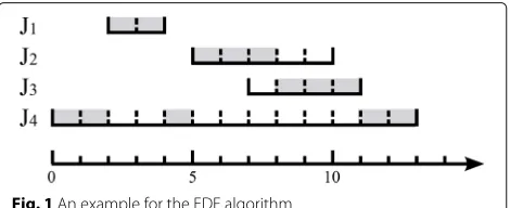
Figure 1 shows an example for the EDF algorithm. In this example, there are four jobs. J1’s processing inter-val is [ 2, 4], and it has two tasks.J2’s processing interval is [ 5, 10], and it has three tasks. J3’s processing interval is [ 7, 11], and it has three tasks.J4’s processing interval is [ 0, 13], and it has five tasks. The EDF algorithm schedules the job with the earliest ending time, and the tasks of a job are always scheduled as early as possible in their process-ing interval. As illustrated in Fig. 1, the gray slots represent the scheduled tasks of the four jobs.
Theorem 1 The EDF algorithm schedules the maximum
number of tasks.
ProofWe prove the theorem by induction. Letn = 1, i.e., there is only one job, then it is easy to find that the EDF algorithm schedules the maximum number of tasks.
Assume the EDF algorithm schedules the maximum number of tasks whenn=k.
Now, we prove that the theorem is correct whenn=k+ 1. If all the tasks ofJk+1can be scheduled in its processing interval, then the theorem is correct. Otherwise, not all the tasks ofJk+1can be scheduled, then there are two cases as follows.
1) If all the scheduled tasks of J1to Jk are within the processing interval [sk+1,ek+1], it indicates thatsk+1 ≤ min1≤i≤k{si}and max1≤i≤k{ei} ≤ ek+1, then all the slots within [sk+1,ek+1] are used.
Fig. 1An example for the EDF algorithm
2) Otherwise, some tasks ofJ1toJkare scheduled before sk+1, and some tasks of J1 to Jk are scheduled within [sk+1,ek+1]. No tasks are scheduled after ek+1 because the ending time max1≤i≤k{ei} ≤ ek+1. We only need to consider whether the scheduled tasks of J1 to Jk within [sk+1,ek+1] can be moved before sk+1. If we can, then more tasks ofJk+1 can be scheduled. However, the EDF algorithm always schedules the tasks as earlier as possible; therefore, it is impossible to move some of these scheduled tasks earlier.
It completes the proof.
For simplicity of illustration, we explain the meaning of linkandreachingwhich will be used frequently later. Both link and reach are defined towards the tasks/jobs which are not dropped (the scheduled tasks/jobs). In this paper, the links are directed.
1) The scheduled tasks of the same job link to each other. We call this the task link.
2) A scheduled jobJilinks to another scheduled job Jj if there exists a scheduled taskT ofJiwhich is scheduled within the processing interval of Jj. We call this the job link and call T the relay task. Figure 2 shows some job link examples. In this figure, the gray slots represent the scheduled tasks. In Fig. 2a,J1 links toJ2since there is a taskTbelonging toJ1which is scheduled within the pro-cessing interval ofJ2. In Fig. 2b,J1andJ2link to each other. Because jobs are scheduled one by one, there may be no task scheduled for the current job. As shown in Fig. 3, no tasks of J3 are scheduled; however,J2 still links toJ3 because taskT ofJ2is scheduled within the processing interval ofJ3.
3) Scheduled task T can reach T belonging to
another job when there exists a job link sequence J(T),Jx1,Jx2. . .,Jxk,J(T)whereJ(T)links toJx1,Jxilinks
toJxi+1, andJxk links toJ(T).J(T)denotes the job
includ-ingT. Figure 4 shows thatJ1can reachJ3. In this example, any scheduled task ofJ1can reach any scheduled task of J3. Reaching is defined for task to task, task to job, and job to job.
Fig. 2 a,bJob link examples
current job, and vice versa. That is, the replacement can also run in a reversed order of the link sequence. In the recursive replacement towards the link sequence, a prior relay task is always replaced with a later relay task.
Algorithm 2EDF-based Algorithm
Input: [si,ei] , ni, uij, 1≤i≤n, 1≤j≤ni
Output: Scheduling the tasks to maximize utility gain 1: Let J1,J2,. . .,Jn be sorted by ending time in
non-decreasing order;
2: Let the tasks of each job be sorted by utility in non-increasing order;
3: fori= 1 tondo 4: forj= 1 tonido
5: ifThere is an unused slot in [si,ei]then
6: Find the earliest unused slot t in [si,ei] and scheduleTijtot;
7: else
8: Find the task with the least utility which can
reachJiand let it beTand its utility beu; 9: ifu<uijthen
10: Run a recursive replacement to removeT;
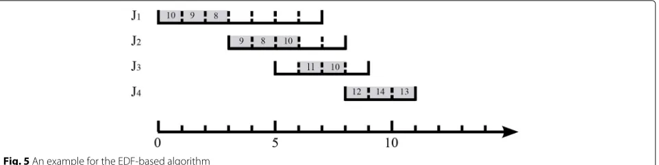
Figure 5 shows an example for the EDF-based algorithm. In this example, there are 4 jobs.J1’s processing interval is [ 0, 7] and it has 5 tasks with utility 10, 9, 8, 7, and 6, respectively.J2’s processing interval is [ 3, 8] , and it has 3 tasks with utility 10, 9, and 8, respectively.J3’s processing interval is [ 5, 9] , and it has 2 tasks with utility 11 and 10, respectively.J4’s processing interval is [ 8, 11] , and it has 3 tasks with utility 14, 13, and 12, respectively. The EDF-based algorithm always schedules the job with the earliest ending time first. In the first iteration, the EDF-based algorithm schedules the 5 tasks ofJ1to slots 1–5, respec-tively. In the second iteration, the EDF-based algorithm schedules the 3 tasks ofJ2to slots 6–8, respectively.
Fig. 3An example for link and reaching
In the third iteration, the EDF-based algorithm sched-ulesJ3’s task with a larger utility of 11 to slot 9, and then, it finds that there is no slot forJ3’s task with smaller utility of 10. The algorithm then finds the task with the small-est utility which can reachJ3. The found task is the task ofJ1, and its utility is 6. In Fig. 6, the red links show a link sequence for the reachability from the task with utility 6 ofJ1 to J3. The tasks pointed by the red arrows are the relay tasks. Every time a relay task is replaced by a later relay task in the link sequence. The algorithm replacesJ1’s task with utility 6 byJ2’s task with utility 8. In the recur-sive replacement,J2’s task with utility 8 is replaced byJ3’s task with utility 10.
In the fourth iteration, the EDF-based algorithm sched-ulesJ4’s tasks with utility 14 and 13 respectively, and then, there is no slot forJ4’s task with utility 12. The algorithm then finds the task with the smallest utility which can reachJ4. The found task is the task ofJ1, and its utility is 7. In Fig. 7, the red links show a link sequence for the reachability from the task with utility 7 ofJ1 to J4. The tasks pointed by the red arrows are the relay tasks. Every time a relay task is replaced by a later relay task in the link sequence. The algorithm replacesJ1’s task with utility 7 byJ2’s task with utility 9. In the recursive replacement, J2’s task with utility 9 is replaced byJ3’s task with utility 11, andJ3’s task with utility 11 is replaced byJ3’s task with utility 12.
The final schedule is shown in Fig. 5. The algorithm schedules the maximum number of tasks achieving the maximum total utility. In Fig. 5, the gray slots have been scheduled with tasks, and the numbers on the gray slots represent task utility.
Theorem 2The EDF-based algorithm is optimal.
ProofTheorem 1 proves that the EDF algorithm sched-ules the maximum number of tasks. We now only need
Fig. 5An example for the EDF-based algorithm
to prove that the EDF-based algorithm maximizes the total utility of the scheduled tasks. We also prove it by induction.
Letn=1, that is, there is only one job. It is easy to find that the EDF-based algorithm maximizes the total utility of the scheduled task because the EDF-based algorithm always schedules the task with the largest utility first.
Assume the EDF-based algorithm maximizes the total utility of the scheduled tasks when there arek jobs, i.e., n=k.
Next, we prove that the theorem is correct whenn =
k+1. Then, we need to prove the EDF-based algorithm
obtains the optimal result forJk+1.
If all the tasks ofJk+1can be scheduled in its processing interval, then the theorem is correct.
Otherwise, if not all the tasks ofJk+1can be scheduled, then the EDF-based algorithm first schedules as many tasks with the largest utility as possible to the unused slots. As stated in Theorem 1, the EDF algorithm can-not schedule more tasks. Therefore, it should determine whether to schedule the remaining tasks of Jk+1or not. For the remaining tasks, the EDF-based algorithm always uses them to replace the tasks with smaller utility. With-out loss of generality, let T be the task with the largest utility in the remaining tasks and its utility be u. LetT be the task with the least utility that has been scheduled, and its utility be u. If u < u, then the largest utility gain is achieved ifT is replaced byT. The utility gain is u−u1+u1−u2+u2−. . .−uk +uk −u = u−u, where{uk,uk−1,. . .,u1}are the utility of the relay tasks in the link sequence fromTtoT. Becauseuis the minimum, u−uis maximum. This property holds for the remaining tasks. It completes the proof.
Fig. 6Third interation, for example Fig. 5
The time complexity of the EDF-based algorithm is O(n2r2), wherenis the number of jobs andris the max-imized number of the tasks of a job. In the EDF-based algorithm, the jobs are scheduled according to the ending time one by one. For the tasks of each job, the algorithm needs to find a task with the smallest utility that has already been scheduled. It needsO(nr)time to search the task in a directed graph constructed by the link relation for tasks to tasks, tasks to jobs, and jobs to jobs. It also needsO(n)time to update the graph any time the graph is changed, i.e. a replacement is implemented.
Ci(s,σ )=min
⎧ ⎪ ⎨ ⎪ ⎩
Ci−1(s,σ )
max{si,Ci−1(s,σ−σi)} +ni
mins,σ{Ci−1(s,σ)+max{0,ni−s+si+Pi−1(s,s,σ−σi−σ)}}
(6)
Pi−1(s,s,σ)=min
Pi−1(s+,s,σ)
min0<σ≤σ{max{0,Ci−1(s,σ)−si+Pi−1(s,s,σ−σ)} (7)
4.2 Problem with only extra job utility
Now, we address the problem where each job has only extra utility and every task does not have utility. If all the tasks of a job are scheduled, then the job obtains the extra utility. Even one task of a job is not scheduled, the job loses the extra utility. This problem is similar to the one studied in [16] where givennjobs with arbitrary processing time, release dates and due dates, and the job can be scheduled
preemptively; the objective is to minimize the sum of the weights of the later jobs. The scheduling of our problem is not preemptive, but the processing time of each task is one unit of time. The preemptive scheduling and a task with one unit of processing time in our problem are sim-ilar. Therefore, minimizing the sum of the weights of the later jobs is the same as maximizing the sum of the utility of the scheduled jobs in our problem. The authors in [16] give a pseudo polynomial time Dynamic Programming (DP) algorithm. We also adopt this algorithm to solve the problem. The DP formulations are represented by Eqs. (6) and (7).
Given a job setJ, lets(J) =minJi∈J{si}be the minimum
starting time ofJ,p(J) = J
i∈Jnibe the total processing
time ofJ,σ (J)=J
i∈Jσibe the total extra utility ofJ, and
c(J)be the time the last job inJis completed in an EDF schedule.
One can refer to article [16] for the detailed algorithm. As stated in that work, assume the jobs are ordered by the ending time in non-decreasing order. Letsbe a starting time, andσ be an integer representing utility. Ci(s,σ )is defined as the minimum value ofc(J)with respect to fea-sible setJ ⊆ {J1,J2,. . .,Ji}, withs(J) ≥ sandσ (J) ≥ σ. If there is no such feasible set J, thenCi(s,σ ) = +∞. Accordingly, the final result that maximizing the weight of a feasible set is given by the largest value ofσ such that Cn(smin,σ )is finite, wheresmin=min1≤i≤n{si}.
If jobJi cannot be contained in a feasible setJ, i.e.si < s(J), thenCi(s,σ )=Ci−1(s,σ ).
Otherwise, if jobJican be contained in the feasible setJ, there exists two cases.
In the first case, job Ji starts after c(J − {Ji}). Either c(J− {Ji})≤si, thenCi(s,σ )= si+ni; orc(J− {Ji}) >si and the scheduled tasks in the interval [si,c(J− {Ji})] are continuous forJ−{Ji}, thenCi(s,σ )=Ci−1(s,σ−σi)+ni. Thus,Ci(s,σ )=max{si,Ci−1(s,σ−σi)} +ni.
In the second case, jobJistarts beforec(J− {Ji}), which indicates there is an idle time betweensiandc(J− {Ji}). LetJbe the last set of jobs scheduled continuously before c(J− {Ji})forJ− {Ji}. Then,c(J)=Ci−1(s(J),σ (J)). Let it bec(J)=Ci−1(s,σ)for simplicity.
Let Pi−1(s,s,σ) be the minimum number of tasks scheduled betweensi ands, with respect to feasible set J ⊆ {J1,J2,. . .,Ji−1} with s(J) ≥ s, c(J) ≤ s, and σ (J)≥σ. Note that it is the minimum number of tasks scheduled in interval [si,s], rather than [s,s]. Then, the number of slots available for jobJibetweensiandscan be represented ass−si−Pi−1(s,s,σ−σi−σ). Thus, the completing timeCi(s,σ )=Ci−1(s,σ)+max{0,ni−s+ si+Pi−1(s,s,σ−σi−σ)}.
Enumerate every s and σ. We can get Ci(s,σ ) = mins>s,σ<σ{Ci−1(s,σ)+max{0,ni−s+si+Pi−1(s,s,σ− σi−σ)}}. The enumeration ofs is among all the start-ing times of the jobs, rather than among all the possible
times, which can drastically reduce the computation complexity.
The computation of Pi−1(s,s,σ) is as follows. Let J ⊆ {J1,J2,. . .,Ji−1} be the set of jobs which realize Pi−1(s,s,σ). Then, there exists two cases.
If s(J) > s, then Pi−1(s,s,σ) = Pi−1(s(J),s,σ). Enumerate everys+>sand find the minimum one, then Pi−1(s,s,σ)=mins+>s{Pi−1(s+,s,σ)}.
Otherwise, if s(J) = s and the scheduling of J is not continuous, let J be the first set of jobs which run
continuously and s(J) = s, then the total
num-ber of tasks scheduled within [si,Ci−1(s,σ (J))] is max{0,Ci−1(s,σ (J)) − si}. We now need to compute the number of tasks which can be scheduled within [Ci−1(s,σ (J)),s]. It is easy to find that Pi−1(s,s,σ) can be represented as max{0,Ci−1(s,σ (J)) − si} + Pi−1(s,s,σ−σ (J)), wheresis the minimum starting time greater than or equal to Ci−1(s,σ (J)). For sim-plicity, let σ = σ (J). Enumerate every σ. We have Pi−1(s,s,σ) = min0<σ≤σ{max{0,Ci−1(s,σ) − si} + Pi−1(s,s,σ−σ)}.
The initial conditions are shown in Eqs. (8) to (11).
C0(s, 0)=s, for all starting times (8)
C0(s,w)= +∞, for all starting timesandw>0 (9)
Pj−1=(s,s, 0)=0, forj=1, 2,. . .,n (10)
P0(s,s,σ)= +∞, forσ>0 (11) The time and space complexities for this DP algorithm areO(n3σ2)andO(n2σ ), respectively, wherenis the num-ber of the jobs andσ is the sum of the utility of the jobs. It can be easily found that the time complexity of the DP algorithm is pseudo polynomial because the DP for-mula includes an integer inputσ which can be extremely large in real systems. Therefore, we provide a theoretical approximation solution for this problem.
4.3 Approximation algorithm for single-machine problem The main idea of the approximation algorithm is to get two intermediate results using the two algorithms inde-pendently and then combine the two results. First, it uses the EDF-based algorithm to solve the problem without extra job utility. Second, it uses the DP algorithm to solve the problem with only extra job utility. Then, it selects a larger one from the two scheduling results. Algorithm APPX1 shows the detailed approximation algorithm.
Theorem 3The APPX1 algorithm is a 2-approximation
algorithm.
ProofLet OPT be the utility obtained by an optimal
Algorithm 3APPX1 algorithm
Input: [si,ei] , σi, ni, uij, 1≤i≤n, 1≤j≤ni Output: Scheduling the tasks to maximize utility gain
1: Use the EDF-based algorithm to solve the problem
without extra utility;
2: Use the DP algorithm to solve the problem with only extra utility;
3: LetT be the set of tasks scheduled by the EDF-based algorithm;
4: LetJ be the set of jobs scheduled by the DP algo-rithm;
5: Letu(T)be the total utility ofT inlcuding the utility of the tasks inT and the extra utility of the completed jobs amongT;
6: Letu(J)be the total utility ofJ including the extra utility of the jobs inJ and the utility of all the tasks of J;
7: ifu(T) <u(J)then
8: Use the scheduling result of the DP algorithm; 9: else
10: Use the scheduling result of the EDF-based
algo-rithm;
algorithm. It is easy to find that OPT can be represented as OPT =u+σ, whereuis the total utility of the sched-uled tasks andσ is the total extra utility of the entirely scheduled jobs in an optimal solution. Letube the total utility obtained by the EDF-based algorithm, andσbe the total utility obtained by the DP algorithm. From the earlier analysis, both the EDF-based algorithm for the problem without extra utility and the DP algorithm for the prob-lem with only extra utility are optimal. Thus,u≤ uand
σ ≤ σ, and then, we have OPT ≤ u +σ. ALG
actu-ally can be represented as ALG ≥max{u,σ}. Therefore,
OPT≤2ALG. It completes the proof.
4.4 An improvement for the DP algorithm
Recall the definition ofCi(s,σ ), it is the minimum value ofc(J)with respect to feasible setJ ⊆ {J1,J2,. . .,Ji}, with s(J) ≥ sandσ (J) ≥ σ. It can be found that, in the DP recursion formulaCi(s,σ ), the parameterσ is build only on the extra utility of the scheduled jobs, but does not consider the utility of the tasks of the scheduled jobs. This can be improved by computingCi(s,u)where the pareme-ter is build on the total utility of the scheduled jobs. Let ui=ni
i=1uij+σi. Useuito replaceσiin the DP formula, thenCi(s,u) represents the minimum value ofc(J) with respect to feasible setJ⊆ {J1,J2,. . .,Ji}, withs(J)≥sand u(J)≥u, whereu(J)includes the utility of all the tasks of the jobs inJand the extra utility of the jobs inJ. Such mod-ification consider the extra utility of the scheduled jobs and also the utility of the tasks of the scheduled jobs. It
can improve the result derived by the DP algorithm when the utility of the tasks takes a large proportion comparing with the extra utility. However, when the extra utility takes a large proportion (for example, in a worst case where all the tasks have no utility, the jobs have only the extra util-ity), the improvement is little. Algorithm APPX1’s use of such modification of the DP algorithm cannot improve the approximation ratio, but may improve the results in many scenarios.
5 Algorithm design for multi-machine problem
The solution for the multi-machine problem is similar to the single-machine problem. It also includes two steps. The first step is to schedule the tasks without consid-ering the extra utility of the jobs. The second step is to schedule the jobs only considering the extra utility of the jobs. And finally, select a better schedule from the two steps.
5.1 Problem without extra utility
The EDF-multi-algorithm is similar to the one for the single-machine problem. The difference is that every time the algorithm needs to schedule a task, it finds the earli-est unused slot in the task’s processing interval among all the machines, while the algorithm for the single-machine problem just needs to search in one machine. If there is no unused slot, the replacement function also finds the task with the smallest utility that has been scheduled among all the machines. The detailed algorithm is shown in Algorithm 4. The obtained result is optimal for the prob-lem without extra utility.
Algorithm 4EDF-Multi algorithm
Input: [si,ei] , ni, uij, 1≤i≤n, 1≤j≤ni
Output: Scheduling the tasks to maximize utility gain 1: Let J1,J2,. . .,Jn be sorted by ending time in
non-decreasing order;
2: Let the tasks of each job be sorted by utility in non-increasing order;
3: fori= 1 tondo 4: forj= 1 tonido
5: ifThere is an unused slot within [si,ei] in some
machinethen
6: Find the earliest unused slottin [si,ei] among all the machines, and let it be machine Mk. ScheduleTijtotat machineMk;
7: else
8: Find the task with the smallest utility that has
been scheduled among all the machines and let it beTand its utility beu;
9: ifu<uijthen
5.2 Problem with only extra utility
We design an algorithm for the multi-machine problem with only extra utility by adopting the idea of the DP algo-rithm for the single-machine problem. Given job set J, let s(J) = minJi∈J{si} be the minimum starting time of is the number of used machines attthat the last job inJis completed in an EDF schedule.
Definet,j+p= t+j+p+m 1,(j+p) modmwhich
represents scheduling p tasks from time t and after
machineMjcontinuously. Because there aremmachines,
m tasks can be scheduled in each slot. We focus on
how many machines are used in slottrather than which machines are used. Without loss of generality, we assume t,jrepresent in slott, machineM1toMjare used. There-fore, the ending time after schedulingptasks from time tand after machineMjcontinuously ist+
all themmachines are used.
Definet,j < t,jift < t ort = tandj < j. It represents that t,j is earlier thant,j.t,j = t,j only ift=tandj=j.
We can regard the scheduling process as putting tasks to a 2-dimensional array from top to bottom and from left to right. Given a starting places,j, the tasks can be sched-uleds,j+1tos,m,s+1, 1tos+1,m,s+2, 1 tos+2,m, and so on. Therefore,t,j − t,j can be regarded as how many tasks can be put fromt,j+1 tot,j.
Let s be a starting time, j be the number of used
machines in s, and σ be an integer representing utility. Similarly to but different from the single-machine prob-lem,Ci(s,j,σ )is defined as the minimum value ofc(J) with respect to feasible setJ⊆ {J1,J2,. . .,Ji}, withs(J)≥s, σ (J)≥σ andjmachines are used ins. If there is no such feasible setJ, thenCi(s,j,σ )= +∞,+∞. Accordingly, the final result maximizing the utility of a feasible set is given by the largest value ofσsuch thatCn(smin, 0,σ )is
The dynamic programming recursion formula is shown in Eqs. (12) and (13). We now introduce the recursion formula in details. The definition of Ci(s, 0,σ ) whose value is a 2-tuple represent the smallest ending place t,xwhere a feasible setJ ⊆ {J1,J2,. . .,Ji}can complete, while satisfyingu(J) ≥ σ, s(J) ≥ s andjmachines are used ins.
IfJi ∈/ J, i.e.,Ji cannot be contained in a feasible setJ satisfying the constraint,Ci(s, 0,σ )=Ci−1(s, 0,σ ).
Let us consider the situationJi∈J, whereJiis contained in a feasible setJsatisfying the constraint. There are two cases as follows. tinuous. That is, some tasks of jobJi can be scatterred betweensi, 0andc(J− {Ji})rather than afterc(J− {Ji}). As stated in [16], the EDF method schedules the tasks as the form of periods of continuous processing. A period of continuous processing is called a block. We consider the scheduling ofJ− {Ji}in the DP algorithm. Let the starting time of the last block inJ− {Ji}bes, 0, and the utility of the last block inJ− {Ji}beσ, then the ending time of the last block isCi−1(s, 0,σ)}. LetPi−1(s, 0,s, 0,σ)be
the minimum amount of processing done betweensi, 0
ands, 0, with respect to feasible setJ⊆ {J1,J2,. . .,Ji−1} We now introduce how to realize the the compu-tation of Pi−1(s, 0,s, 0,σ). Recall the definition of every s+ > s and find the result. The result is the minimum one among mins+>s{Pi−1(s+, 0,s, 0,σ)}.
Otherwise, s(J), 0 = s, 0. Let the first block in the solution beJ and the total extra utility of the first
block be σ, then the ending time of the first block
be represented as max{0,Ci−1(s, 0,σ) − si, 0} + Pi−1(s, 0,s, 0,σ − σ), where s is the smallest starting time s, 0 ≥ Ci−1(s, 0,σ). Enumerat-ing every σ, we can obtain Pi−1(s, 0,s, 0,σ) = min0<σ≤σ{max{0,Ci−1(s, 0,σ) − si, 0} + Pi−1(s, 0,s, 0,σ−σ)}.
The initial conditions are shown in Eqs. (14) to (17).
C0(s, 0, 0)=
s+1 m
,smodm
, for all starting times
(14)
C0(s, 0,w)= +∞, for all starting timesandw>0 (15)
Pj−1=(s, 0,s, 0, 0)=0, forj=1, 2,. . .,n (16)
P0(s, 0,s, 0,σ)= +∞, forσ>0 (17)
An improvement of the DP formula for the single-machine problem can also be used in the multi-single-machine problem. It cannot improve the result in a worst case where the tasks have no utility, but it can improve the result for many inputs.
5.3 Approximation algorithm for multi-machine problem The same as single-machine problem, the main idea of the approximation algorithm for the multi-machine problem is to get two intermediate results using the EDF-algorithms and the DP algorithm for the multi-machine problem independently and then combine the two results of the two algorithms. First, it uses the EDF-multi-algorithm to solve the problem without extra job utility. Second, it uses the DP algorithm to solve the prob-lem with only extra job utility. Finally, it selects a larger one from the two scheduling results. Algorithm APPXm shows the detailed approximation algorithm.
Theorem 4 The APPXm algorithm is a 2-approximation
algorithm.
Proof Let OPT be the utility obtained by an optimal
solution and ALG be the utility obtained by the APPXm
algorithm. It is easy to find that OPTcan be represented as OPT=u+σ, whereuis the total utility of the scheduled tasks andσ is the total extra utility of the entirely sched-uled jobs in an optimal solution. Letube the total utility derived by the EDF-multi-algorithm and σ be the total utility obtained by the dynamic programming algorithm. From the earlier analysis, both the EDF-multi-algorithm for the problem without extra utility and the dynamic pro-gramming algorithm for the problem with only an extra utility are optimal. Thus, u ≤ u andσ ≤ σ, then we have OPT ≤u+σ. ALGactually can be represented as
Algorithm 5APPXm algorithm
Input:m,n, [si,ei] ,σi, ni, uij, 1≤i≤n, 1≤j≤ni Output: Scheduling the tasks tommachines to maximize utility gain.
1: Use the EDF-Multi algorithm to solve the problem
without extra utility;
2: Use the dynamic programming algorithm to schedule
jobs with only the extra utility tommachines;
3: Use the EDF-Multi algorithm to solve the problem
without extra utility;
4: Use the DP algorithm to solve the problem with only extra utility;
5: LetT be the set of tasks scheduled by the EDF-Multi algorithm;
6: LetJ be the set of jobs scheduled by the DP algo-rithm;
7: Letu(T)be the total utility ofT inlcuding the utility of the tasks inT and the extra utility of the completed jobs amongT;
8: Letu(J)be the total utility ofJ including the extra utility of the jobs inJ and the utility of all the tasks of J;
9: ifu(T) <u(J)then
10: Use the scheduling of the DP algorithm; 11: else
12: Use the scheduling of the EDF-Multi algorithm;
ALG≥max{u,σ}. Therefore, OPT≤2ALG. It completes the proof.
6 Simulation result
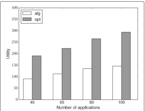
The simulation result is shown in this section. As the com-putation complexity of our algorithm is high, especially the DP algorithm; thus, the input of our simulation is set to not too large. The number of machines used in our simulation is at most 5, the number of applications is at most 100, and the number of tasks for each application is at most 5. The utility of each task is a random value. The starting time and the ending time and the extra utility of each application is also randomly generated.
As the optimal result is hard to compute; thus, we use an upper bound result to represent the optimal result. The upper bound is computed by dividing the extra utility of each application into its tasks in proportion, that is task with high utility will be assigned with a high extra utility.
Fig. 8Scheduling with single machine
the single machine is approaching to its maximum com-puting load. Figure 9 illustrates the scheduling result in five machines. Similar as the single-machine case, the util-ity that the approximation algorithm can get increase as the number of applications increases. And the increasing rate gets slower as the multiple machines are getting to their maximum load. Because the upper bound we used to represent the optimal result is higher than the real opti-mal result, therefore, the utility that the approximation algorithm gets can get closer to the optimal result and the difference is much less than two times, which confirms the approximation ratio; thus, the performance is acceptable in our simulation.
7 Conclusions
This paper proposes a class of algorithms to solve the problem of maximizing utility for job scheduling where each job consists of multiple tasks. Different from the
Fig. 9Scheduling with multi-machine
existing works which either consider job utility or task utility individually, this paper considers both job util-ity and task utilutil-ity simultaneously by introducing extra utility for every job. We analyze the complexity of the problem and discuss two sub-problems of scheduling jobs in a single machine and scheduling jobs in multiple machines. We design two 2-approximation algorithms for the sub-problems, and the approximation proofs are also presented. Although the time complexity is pseudo poly-nomial, we provide a theoretical insight into this problem.
Acknowledgements
This work was supported in part by the National Natural Science Foundation of China under grant nos. 61502099, 61632008, 61320106007, 61502100, 61532013, 61602084, and 61672154, Jiangsu Provincial Natural Science Foundation of China under grant no. BK20150637, Jiangsu Provincial Key Laboratory of Network and Information Security under grant no. BM2003201, Key Laboratory of Computer Network and Information Integration of Ministry of Education of China under grant no. 93K-9, and Collaborative Innovation Center of Novel Software Technology and Industrialization.
Authors’ contributions
XF and WW conceived and designed the study. XF performed the experiments. XF and YL wrote the paper. JL, HG, and YL reviewed and edited the manuscript. All authors read and approved the final manuscript.
Competing interests
The authors declare that they have no competing interests.
Publisher’s Note
Springer Nature remains neutral with regard to jurisdictional claims in published maps and institutional affiliations.
Author details
1School of Computer Science and Engineering, Southeast University, Nanjing,
China.2School of Computer Science and Technology, Harbin Institute of
Technology, Harbin, China.3Department of Computer Science, Georgia State
University, Atlanta, USA.
Received: 10 August 2017 Accepted: 13 November 2017
References
1. SH Bokhari,Assignment Problems in Parallel and Distributed Computing,vol. 32. (Springer US, New York, 2012)
2. M Armbrust, A Fox, R Griffith, AD Joseph, R Katz, A Konwinski, et al., A view of cloud computing. Commun. ACM.53(4), 50–58 (2010). Available from: URL http://doi.acm.org/10.1145/1721654.1721672
3. Q Zhang, L Cheng, R Boutaba, Cloud computing: state-of-the-art and research challenges. J. Int. Serv. Appl.1(1), 7–18 (2010). Available from: http://dx.doi.org/10.1007/s13174-010-0007-6
4. V Sharma, U Mukherji, V Joseph, S. Gupta, Optimal energy management policies for energy harvesting sensor nodes. IEEE Trans. Wirel. Commun.
9(4), 1326–1336 (2010)
5. C Lefurgy, K Rajamani, F Rawson, W Felter, M Kistler, TW Keller, Energy management for commercial servers. Computer.36(12), 39–48 (2003) 6. RL Graham, EL Lawler, JK Lenstra, AHGR Kan, inDiscrete Optimization
IIProceedings of the Advanced Research Institute on Discrete Optimization and Systems Applications of the Systems Science Panel of NATO and of the Discrete Optimization Symposium co-sponsored by IBM Canada and SIAM Banff, Aha. and Vancouver. vol. 5 of Annals of Discrete Mathematics, ed. by ELJ P L Hammer, BH Korte. Optimization and approximation in deterministic sequencing and scheduling: a survey (Elsevier, 1979), pp. 287–326. Available from: http://www.sciencedirect.com/science/ article/pii/S016750600870356X. Accessed 29 Apr 2008
8. EL Lawler, JK Lenstra, AHGR Kan, DB Shmoys, inLogistics of Production and Inventory. vol. 4 of Handbooks in Operations Research and Management Science. Chapter 9. Sequencing and scheduling: algorithms and complexity (Elsevier, 1993), pp. 445–522. Available from: http://www. sciencedirect.com/science/article/pii/S0927050705801896 9. J Blazewicz, JK Lenstra, AHGR Kan, Scheduling subject to resource
constraints: classification and complexity. Discret. Appl. Math.5(1), 11–24 (1983). Available from: http://www.sciencedirect.com/science/article/pii/ 0166218X83900124. Accessed 9 Sept 2002
10. Y Zheng, B Ji, N Shroff, P Sinha, in2015 IEEE 8th International Conference on Cloud Computing. Forget the deadline: scheduling interactive
applications in data centers (IEEE, New York, 2015), pp. 293–300 11. MR Garey, DS Johnson, Two-processor scheduling with start-times and
deadlines. SIAM J. Comput.6(3), 416–426 (1977)
12. MR Garey, DS Johnson,Computers and Intractability: A Guide to the Theory of NP-Completeness. (W.H. Freeman & Co, New York, 1979)
13. A Bar-Noy, S Guha, JS Naor, B Schieber, inProceedings of the Thirty-first Annual ACM Symposium on Theory of Computing. STOC ’99. Approximating the throughput of multiple machines under real-time scheduling (ACM, New York, 1999), pp. 622–631. Available from: http://doi.acm.org/10. 1145/301250.301420
14. A Bar-Noy, R Bar-Yehuda, A Freund, J (Seffi) Naor, B Schieber, A unified approach to approximating resource allocation and scheduling. J. ACM.
48(5), 1069–1090 (2001). Available from: http://doi.acm.org/10.1145/ 502102.502107
15. G Calinescu, A Chakrabarti, H Karloff, Y Rabani, An improved
approximation algorithm for resource allocation. ACM Trans. Algorithms.
7(4), 48:1–48:7 (2011). Available from: http://doi.acm.org/10.1145/ 2000807.2000816
16. EL Lawler, A dynamic programming algorithm for preemptive scheduling of a single machine to minimize the number of late jobs. Ann. Oper. Res.
26(1-4), 125–133 (1991). Available from: http://dx.doi.org/10.1007/ BF02248588
17. G Steiner, Models and algorithms for planning and scheduling problems minimizing the number of tardy jobs with precedence constraints and agreeable due dates. Discret. Appl. Math.72(1), 167–177 (1997). Available from: http://www.sciencedirect.com/science/article/pii/
S0166218X96000431. Accessed 10 Jan
18. H Kise, T Ibaraki, H Mine, A solvable case of the one-machine scheduling problem with ready and due times. Oper. Res.26(1), 121–126 (1978). Available from: http://dx.doi.org/10.1287/opre.26.1.121
19. V Bafna, B Narayanan, R6 Ravi,Nonoverlapping Local Alignments, Weighted Independent Sets of Axis Parallel Rectangles. (Center for Discrete Mathematics & Theoretical Computer Science, Princeton, 1995) 20. P Berman, B DasGupta, S Muthukrishnan, inProceedings of the Thirteenth
Annual ACM-SIAM Symposium on Discrete Algorithms. SODA ’02. Simple approximation algorithm for nonoverlapping local alignments (Society for Industrial and Applied Mathematics, Philadelphia, 2002), pp. 677–678. Available from: http://dl.acm.org/citation.cfm?id=545381.545471 21. R Bar-Yehuda, MM Halldórsson, JS Naor, H Shachnai, I Shapira, in
Proceedings of the Thirteenth Annual ACM-SIAM Symposium on Discrete Algorithms. SODA ’02. Scheduling split intervals (Society for Industrial and Applied Mathematics, Philadelphia, 2002), pp. 732–741. Available from: http://dl.acm.org/citation.cfm?id=545381.545479
22. R Bar-Yehuda, D Rawitz, Using fractional primal-dual to schedule split intervals with demands. Discret. Optim.3(4), 275–287 (2006). Available from: http://dx.doi.org/10.1016/j.disopt.2006.05.010