Weighted exponential stability for generalized delay functional differential equations with bounded delays

R E S E A R C H

Open Access

Weighted exponential stability for

generalized delay functional differential

equations with bounded delays

Snezhana Hristova

1*

_{and Valentina Proytcheva}

2

*_{Correspondence:}

[email protected]

1_{Plovdiv University, Plovdiv, Bulgaria}

Full list of author information is available at the end of the article

Abstract

In the paper functional differential equations with several bounded delays are considered. The delays are presented in the form of delay operators and they generalize many well-known types of delay differential equations in the literature, such as differential equations with constant delays, with variable delays, with distributed delays, differential equations with maxima,etc.A special type of stability, known as

ψ

-exponential stability, is studied and several sufficient conditions are obtained. The used function

ψ

plays the role of a weight in the norm and,

additionally, it gives the rate of increase of the solutions which are not exponentially stable in the regular sense. The modified Razumikhin method as well as comparison results have been applied. Several examples illustrate the results obtained.

MSC: 34K20

Keywords: exponential stability with weight; Lyapunov function; delay; differential equations

1 Introduction

One of the main qualitative questions in the theory of differential equations is stability. The problems of the stability of the solutions of differential equations via Lyapunov functions have been successfully investigated and various types of stability have been introduced. One of the useful types of stability is the so-called exponential stability. In [, ] the au-thors have investigated the exponential stability of impulsive delay differential equations by using the method of Lyapunov functions and by Razumikhin techniques.

The exponential stability gives information as regards the rate of decay of the solutions only in the case when the solutions are stable. But often the solutions are not bounded at all, or they are bounded but not exponentially stable. In this case we could apply a weight such that the solution could become exponentially stable in a different sense. We could introduce and use the so-calledψ-stability. The notion ofψ-stability of degreek

for ordinary differential equations has been introduced by Akinyele []. Also various types ofψ-stability have been studied for nonlinear systems of ordinary differential equations [], for nonlinear Volterra integro-differential systems [], for impulsive differential equa-tions []. Meanwhile, in [] points inRn_{are incorrectly mixed with values of functions}

with a rangeRn_{and the weights in the examples are useless.}

In the mathematical simulation in various important branches of control theory, phar-macokinetics, economics,etc., one has to analyze the influence of the deviation of the reg-ulated quantity. Such a kind of problems could be adequately modeled by differential equa-tions that contain a delay operator. In this paper differential equaequa-tions with a special type of delay operators are considered. These delay equations generalize many types of equa-tions well known in the literature. Several sufficient condiequa-tions for theψ-exponential sta-bility by scalar Lyapunov functions are obtained. The modified Razumikhin method and comparison results have been applied. Several examples, solved and graphed by Wolfram Mathematica, are given to illustrate the main concepts of the weighted exponential stabil-ity.

2 Preliminary notes and definitions

Letr>  be a given number. Define the operatorsGk:C([–r,∞),Rn)→Rn,k= , , . . . ,m,

such that for any functionx∈C([–r,∞),Rn_{), any pointt∈R}

+, andk= , , . . . ,m, there

exists a pointξ∈[t–r,t], depending onx,t,k, such thatGk(x)(t) =Cx(ξ), whereCis a

constant.

Consider the nonlinear generalized delay functional differential equations with bounded delays

x=ft,x(t),G(x)(t),G(x)(t), . . . ,Gm(x)(t)

fort≥t, ()

with initial condition

x(t+t) =ϕ(t) fort∈[–r, ], ()

wherex∈Rn_,f:R

+×Rn×Rnm→Rn,t∈R+,ϕ: [–r, ]→Rn.

We would like to emphasize some particular cases of ():

- if for any pointt∈R+the pointξk∈Ris such thatξk=t–hk,k= , , . . . ,m, where hk= const∈[,r],k= , , . . . ,m, thenGk(x)(t) =x(t–hk)fort∈R+and () is reduced to the delay differential equations with constant delays, well known and studied in the literature,x=f(t,x(t),x(t–h),x(t–h), . . . ,x(t–hm));

- if for any pointt∈R+the pointξk∈Ris such thatmaxs∈[t–hk,t]x(s) =x(ξk),

hk= const∈[,r],k= , , . . . ,m, thenGk(x)(t) =maxs∈[t–hk,t]x(s)fort∈R+and () is reduced to differential equations with maxima, which are partially studied in [–], see also the monograph [] and the references cited therein:

x=f

t,x(t), max

s∈[t–h,t]x(s),s∈max[t–h,t]x(s), . . . ,s∈max[t–hm,t] x(s)

;

- if for any pointt∈R+the pointξk∈Ris such thatξk=t–τk(t), where the functions

τk:R+→[,r], thenGk(x)(t) =x(t–τk(t))fort∈R+and () is reduced to the delay differential equations with variable bounded delays, well known and studied in the literature:x=f(t,x(t),x(t–τ(t)),x(t–τ(t)), . . . ,x(t–τm(t)))(for example,

τ(t) =r|sin(t)|orτ(t) =_trt_+ fort∈R+).

In our work we will assume that IVP (), () (initial value problem) has a solution

In our investigations we will use a special function, which will play the role of the weight in the regular norm inRn_{and it will help us to generalize the well-known exponential}

stability. Letψk: [–r,∞)→(,∞),k= , , . . . ,n, be given continuous functions and letψ

be an×n-dimensional matrix defined byψ=diag[ψ,ψ, . . . ,ψn].

We will define exponential stability with a weight for generalized nonlinear delay func-tional differential equations ().

Definition  Let the functionsψk∈C([–r,∞), (,∞)),k= , , . . . ,n, be given. The zero

solution of the system of generalized delay functional differential equations () is said to be:

() ψ-exponentially stable, if for any initial pointt∈R+and any initial function

ϕ∈C([–r, ],Rn_{)there existβ=β(t) > and a constantδ> such that the} solutionx(t;t,ϕ)of IVP (), () satisfies

ψ(t)x(t;t,ϕ)≤β(t)ψ ϕt_e–δ(t–t), t≥t,

whereψ ϕt_=maxs∈[t–r,t]ψ(s)ϕ(s–t);

() ψ-uniformly exponentially stable, ifβin () does not depend ont.

Remark  The definition of stability given above generalizes the exponential stability, well

known in the literature (ifψk(t)≡ fork= , , . . . ,n).

Remark  If the weight functionψis one-to-one, then we could consider the substitution

y(t) =ψ(t)x(t), wherex(t) is a solution of (), and study the exponential stability ofy(t) which is equivalent to theψ-exponential stability ofx(t). But if the functionψ(t) is not a one-to-one function, then we have to study directly the behavior of the solution ().

Theψ-exponential stability defined above is often used in connection with the rate of increase/decrease of unbounded solutions.

Definition  The rate of increase of a functionu: [a,∞)→Rn_{is smaller than the}

func-tionη∈C([a,∞), (,∞)) if there existsC=C(a,u(a)) >  such thatu(t)<Cη(t) for

t≥a.

Remark  If the zero solution of () is exponentially stable,i.e.

x(t;t,ϕ)<β(t)ϕt_e–δ(t–t), t≥t,

then any solution of () has a rate of increase smaller thane–δt_{, whereC=β(t)ϕt} e

δt_.

Remark  If the solutions of () are unbounded but the zero solution is weighted expo-nentially stable, then with the help of the weight we could easily obtain the rate of increase of the solutions.

solution of the equation could be more difficult than the study of theψ-exponential stabil-ity of the given one. That is why it requires directly studying of theψ-exponential stability and obtaining of appropriate sufficient conditions.

Example  Consider the delay differential equation

x(t) =x(t– ) fort≥ ()

with an initial condition

x(t+ ) =ϕ(t) fort∈[–, ], ()

wherex∈R,ϕ∈C([–, ],R).

Letϕ(t) =t_{fort∈[–, ]. Then the solutionx(t) is unbounded.}

Consider the functionψ(t) = –.t. Then the functiony(t) = –.tx(t) satisfiesy(t) = –.y(t) + –._{y(t– ), which is more complicated than the given equation (). That is}

why it is better to study directly theψ-exponential stability of the zero solution of () (see Figure ). Also, we could find the rate of increase ofx(t) which is smaller than the function .t_e–.t_{(see Figure ).}

Figure 1 Graph of|2–1.22t_{x(t)|and 1.2e}–0.22t_{on [2, 30].}

Figure 3 Graph of|(t– 3)2_e–t_{x(t)|and 1.5e}–0.05t_{on [2, 80].}

Figure 4 Graph of (t– 3)2_e–t_{on [2, 10].}

Now let the function ψ(t) = (t– )_e–t_{. Obviously the function y(t) =ψ(t)x(t)}

satis-fies a more complicated equation. We directly graph the functionsψ(t)x(t) and .e–.t

wherex(t) is the solution of () (see Figure ). The zero solution could be{(t– )_e–t_}

-exponentially stable. In this case, since the function ψ(t) is not a one-to-one function (Figure ) we are not able to find directly the rate of increase ofx(t).

We will use Lyapunov functions and the Razumikhin method to obtain some sufficient conditions for theψ-exponential stability of the zero solution of (). We will apply the differentiable Lyapunov functionV(t,x) and we will define for anyt∈R+and any function ∈C([–r, ],Rn_{) a derivative ofV(t,x) along a trajectory of the system () with a weight}

ψ as follows:

D()Vt,ψ(t) ()

=∂V(t,ψ(t) ()) ∂t

+∂V(t,ψ(t) ()) ∂x

ψ(t) ()

+ψ(t)ft, (),G( )(),G( )(), . . . ,Gm( )()

,

3 Main results

We will obtain some sufficient conditions for the weighted exponential stability of nonlin-ear generalized delay functional differential equations.

Then the zero solution of the generalized delay functional differential equation ()is

ψ-exponentially stable.

We will prove the functionQ(t) to be non-positive.

Fors∈[t–t∗, ) andt∗>twe get

According to the proved inequalities in Case  and Case  it follows that the inequality in condition (ii) is satisfied for the function φ(s) =x(t∗+s),s∈[–r, ]. Therefore, from

The proof of Theorem  is completed.

Remark  Note that the functionw(t) in inequality () could be replaced by a positive constantC.

Corollary  Let there exist positive constants A,B,C,p such that a(t)≡A,b(t)≡B,w(t)≡

Then the zero solution of the generalized delay functional differential equation ()is

ψ-uniformly exponentially stable.

In the case when the weight is involved in the derivative of the Lyapunov function we obtain the following sufficient conditions for theψ-exponential stability.

Theorem  Let there exist a Lyapunov function V∈C([–r,∞)×Rn,R+),functions a,b:

[–r,∞)→R+,w:R+→(,∞),and a positive constant p such thatinft≥w(t) =C> ,

inft≥a(t) =A> ,and

(i) a(t)xp_{≤V(t,x)≤b(t)x}p_{fort∈[–r,∞),x∈R}n_;

(ii) for any numbert∈R+and any functionφ∈C([–r, ],Rn)such that V(t,ψ(t)φ())≥e–_tt_–rw(s)ds_{V(t+s,ψ(t+s)φ(s))fors∈[–r, )the inequality}

D()V

t,ψ(t)φ()< –w(t)Vt,ψ(t)φ()

holds.

Then the zero solution of the generalized delay functional differential equation ()is

ψ-exponentially stable.

Proof The proof of Theorem  is similar to the one of Theorem , but the functionQ(t) is defined by

Q(t) =

⎧ ⎨ ⎩

V(t,ψ(t)x(t)) –M(t)(ψ ϕt)

p_e–tt_w(s)ds _fort≥_t ,

V(t,ψ(t)ϕ(t–t)) –M(t)(ψ ϕt_)p _{fort∈[t–r,t].}

Remark  The functionw(t) under the conditions of Theorem  and Theorem  could not vanish, so in the case when the derivative of the Lyapunov function is strongly negative, we need another type of sufficient condition.

Theorem  Let there exist a Lyapunov function V∈C([–r,∞)×Rn,R+),functions a,b:

[–r,∞)→R+:inft≥a(t) =A> ,and positive constantsγ∈(, )and p> such that (i) a(t)xp_{≤V(t,x)≤b(t)x}p_forx∈Rn_;

(ii) for any numbert∈R+and any functionφ∈C([–r, ],Rn)such that V(t,ψ(t)φ()) >γV(t+s,ψ(t+s)φ(s))fors∈[–r, )the inequality

D()V

t,ψ(t)φ()< 

holds.

Then the zero solution of the generalized delay functional differential equation ()is

ψ-exponentially stable.

Proof Letx(t) =x(t;t,ϕ) be a solution of IVP (), (). Choose a positive numberλ:λ< –ln_rγ. Thenγeλr_{< .}

Define a functionv: [t–r,∞)→R+byv(t) =V(t,ψ(t)x(t)). We will prove

v(t)≤M(t)ψ ϕp_te–λ(t–t), t≥t–r, ()

Lett∈[t–r,t]. From condition (i) it follows thatv(t) =V(t,ψ(t)x(t))≤b(t)(ψ(t)ϕ(t–

t))p_{≤M(t)ψ ϕ}p t≤e

–λ(t–t)_{M(t)ψ ϕ}p t.

Assume the contrary and let

t∗=supt>t:v(s)≤M(t)ψ ϕp_te–λ(t–t)fors∈[t,t].

It is obvious thatt∗<∞,v(t∗)≤M(t)ψ ϕp_te–λ(t∗–t)_and

vt∗≥. ()

Lets∈[–r, ). Then we have

γVt∗+s,ψt∗+sxt∗+s

=γvt∗+s≤γM(t)ψ ϕp_te–λ(t∗+s–t)

≤γeγrM(t)ψ ϕp_te–λ(t∗–t)

=γeλrvt∗<Vt∗,ψt∗xt∗.

Therefore, from (ii) we getD()V(t∗,ψ(t∗)x(t∗)) < , which contradicts (). From inequality () and condition (i) it follows that

ψ(x)x(t)≤ p

V(t,ψ(t)x(t))

a(t) ≤

p

M(t)

a(t)

ψ ϕt_e–λp(t–t)

≤ p

M(t)

A

ψ ϕt_e–λp(t–t) _fort≥_t

. ()

The proof of Theorem  is completed.

Corollary  Let conditions of Theorem/Theorem be satisfied for a(t)≡A>  and b(t)≡b> .

Then the zero solution of the generalized delay functional differential equation ()is

ψ-uniformly exponentially stable.

4 Applications

Now we will give some examples to illustrate the theoretical result obtained.

Example  Consider again the delay differential equation (). We will prove theoretically that the zero solution of () isψ-uniformly exponentially stable, whereψ(t) = –.t_.

LetV(x) = .x_{. It is easy to check the validity of condition (i) of Theorem  forp= ,} a(t)≡,b(t)≡.

Now let t ∈ R+ and φ ∈ C([–, ],R) be such that V(ψ(t)φ()) > .V(ψ(t)φ(s))

for s ∈ [–, ) or (φ()) _{> .(}–.s_φ(s))_{. Then applying the inequalities (φ())} _>

.(._φ(–))_{andab≤.(a}_+b_{), we obtain the following inequality:}

D()Vψ(t)φ()= –.t–.ln() + .φ()+ .φ(–)

According to Theorem  the zero solution of () isψ-uniformly exponentially stable,i.e.

Example  Consider the following system of differential equations with maxima:

x(t) =y(t) –x(t),

Note that it is not possible to obtain the solutions of the system () in an explicit form. So, we will use the results obtained above to draw a conclusion about the behavior of the solutions.

According to Theorem  the zero solution of () isψ-exponentially stable. From in-equality () we obtain

Inequality () proves that the zero solution of () is also exponentially stable.

Figure 5 The graph of the solutionx(t),y(t) of (16), (17).

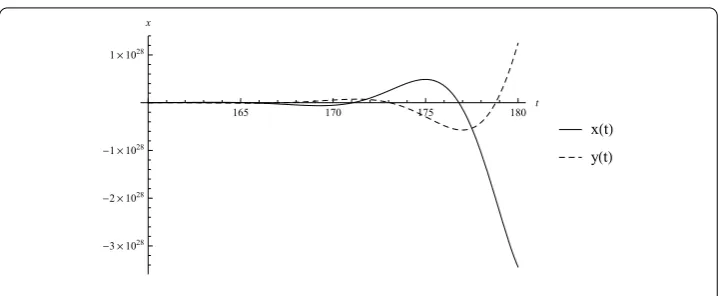
Example  Consider the following system of delay differential equations:

x(t) =y(t) +x(t– ) +y(t– ),

y(t) = –x(t) +x(t– ) +y(t– ) fort≥

()

with initial condition

x(t+s) =φ(s), y(t+s) =φ(s) fors∈[–, ], ()

wherex,y∈R.

We use Wolfram Mathematica to obtain numerically the solutionx(t),y(t) of IVP (), () fort= ,φ(t) = ,φ(t) = ,t∈[–, ] and we graph it (Figure ). It is obvious that

the zero solution is not exponentially stable.

Applying the above results we will prove theψ-exponential stability of the zero solution of (), whereψ(t) = (ψ(t),ψ(t)),ψ(t) =ψ(t) =e–t.

ConsiderV(t,x,y) = .(x_+y_{). Then the condition (i) of Theorem  is satisfied for} p= ,a(t)≡ andb(t) = .

For any t∈R+ and any function φ∈C([–, ],R), φ = (φ,φ) such that (φ())+

(φ())> .((φ(s))+ (φ(s))) fors∈[–, ), we use the inequality ab≤a+b and

obtain

D()Vt,ψ(t)φ()

=e–tφ()

φ()

+φ()φ(–) +φ()φ(–)

–φ()

φ()

+φ()φ(–) +φ()φ(–)

– e–tφ() 

+φ() 

≤e–t–φ()+φ()

+φ(–)+φ(–)

< . ()

According to Theorem  the zero solution of () isψ-uniformly exponentially stable and inequality () is satisfied,i.e.

ψ(t)u(t)≤ψ ϕt_e–.(t–t) fort≥t, ()

Figure 6 The graph ofe–6t(|x(t)|+|y(t)|) – 2e6e–0.25ton [60, 100].

Figure 7 The graphs ofe–6t_{(|x(t)|+|y(t)|) and 2e}–0.25t_{on [0, 30].}

Figure 8 The graph ofe–6t(|˜x(t)|+|˜y(t)|) – 150e–174e–0.25(t–30)on [30, 100].

From inequality () it follows thatu(t) ≤e–.t+ϕt_e.t,i.e.the rate of increase of any solution of () is smaller thane.t.

In the particular case of the initial conditiont= ,φ(t) = ,φ(t) = ,t∈[–, ],

in-equality () is reduced toψ(t)U(t) ≤ee–.t, andU= (x,y),x(t),y(t) is the solution of (), (). From Figure  it is seen that inequality () is true.

Now use the functionψ(t) = (ψ(t),ψ(t)),ψ(t) =ψ(t) =e–t as a weight and graph

Consider the delay equation () with initial condition

x(t) = , y(t) = – fort∈[, ]. ()

For the initial value problem (), () inequality () is reduced to ψ(t)u˜(t) ≤ e–_e–.(t–)_{,u˜ = (x˜,˜y), where the couple of functions (x˜(t),y˜(t)) is the solution of}

(), (). From Figure  it is seen that inequality () is true.

Competing interests

The authors declare that they have no competing interests.

Authors’ contributions

All the authors contributed equally to this work. They all read and approved the final version of the manuscript.

Author details

1_{Plovdiv University, Plovdiv, Bulgaria.}2_{Technical University of Sofia, Branch Plovdiv, Plovdiv, Bulgaria.}

Acknowledgements

The research was partially supported by Project BG051PO001/3.3-05- 001 Science and Business, financed by the Operative Program, Development of Human Resources, European Social Fund and Fund Scientific Research MU13FMI002, Plovdiv University.

Received: 10 May 2014 Accepted: 4 June 2014 Published:22 Jul 2014

References

1. Wang, Q, Zhu, Q: Razumikhin-type stability criteria for differential equations with delayed impulses. Electron. J. Qual. Theory Differ. Equ.2013, 14 (2013)

2. Zhang, GL, Song, MH, Liu, MZ: Exponential stability of impulsive delay differential equations. Abstr. Appl. Anal.2013, Article ID 938027 (2013). doi:10.1155/2013/938027

3. Akinyele, O: On partial stability and boundedness of degreek. Atti Accad. Naz. Lincei, Rend. Cl. Sci. Fis. Mat. Nat. (8)

65(6), 259-264 (1978)

4. Morchalo, J: On (ψ-Lp)-stability of nonlinear systems of differential equations. An. ¸Stiin¸t. Univ. ‘Al.I. Cuza’ Ia¸si, Mat.

36(4), 353-360 (1990)

5. Dimandescu, A: On theψ-stability of nonlinear Volterra integro-differential systems. Electron. J. Differ. Equ.2005, 56 (2005)

6. Gupta, B, Srivastava, SK:ψ-Exponential stability for non-linear impulsive differential equations. Int. J. Comput. Math. Sci.4(7), 329-333 (2010)

7. Agarwal, RP, Hristova, S: Strict stability in terms of two measures for impulsive differential equations with ‘supremum’. Appl. Anal.91(7), 1379-1392 (2012)

8. Dishliev, A, Hristova, S: Stability on a cone in terms of two measures for differential equations with ‘maxima’. Ann. Funct. Anal.1(1), 133-143 (2010)

9. Henderson, J, Hristova, S: Eventual practical stability and cone valued Lyapunov functions for differential equations with ‘maxima’. Commun. Appl. Anal.14(4), 515-524 (2010)

10. Hristova, S: Lipschitz stability for impulsive differential equations with ‘supremum’. Int. Electron. J. Pure Appl. Math.

1(4), 345-358 (2010)

11. Hristova, S: Practical stability and cone valued Lyapunov functions for differential equations with ‘maxima’. Int. J. Pure Appl. Math.57(3), 313-324 (2009)

12. Hristova, S: Stability on a cone in terms of two measures for impulsive differential equations with ‘supremum’. Appl. Math. Lett.23, 508-511 (2010)

13. Hristova, S, Gluhcheva, S: Lipschitz stability in terms of two measures for differential equations with ‘maxima’. Int. Electron. J. Pure Appl. Math.2(2), 1-12 (2010)

14. Bainov, D, Hristova, S: Differential Equations with ‘Maxima’. CRC Press, Boca Raton (2011)

10.1186/1687-1847-2014-185