An effective collocation technique to solve the singular Fredholm integral equations with Cauchy kernel

(1)

R E S E A R C H

Open Access

An effective collocation technique to

solve the singular Fredholm integral

equations with Cauchy kernel

Ali Seiﬁ, Taher Lotﬁ

*

_{, Toﬁgh Allahviranloo and Mahmoud Paripour}

*_{Correspondence:} lotﬁ[email protected] Department of Mathematics, Islamic Azad University, Hamedan Branch, Hamedan, Iran

Abstract

In this paper, an effective numerical method to solve the Cauchy type singular Fredholm integral equations (CSFIEs) of the first kind is proposed. The collocation technique based on Bernstein polynomials is used for approximation the solution of various cases of CSFIEs. By transforming the problem into systems of linear algebraic equations, we see that this approach is computationally simple and attractive. Then the approximate solution of the problem in truncated series form is obtained by using the matrix form of this method. Convergence and error analyses of the presented method are mentioned. Finally, numerical experiments show the validity, accuracy, and efficiency of the proposed method.

Keywords: collocation method; singular integral equation; Cauchy kernel; Bernstein polynomial

1 Introduction

The concept of the principal value of a Cauchy type singular integral equation is well known. This kind of equations is applied in many branches of engineering and science like fracture mechanics [], aerodynamics [] and occurs in a variety of mixed boundary value problems of mathematical physics [–]. The Cauchy singular integral equations form is given as



–

y(t)

t–sdt+



–

k(s,t)y(t)dt=g(s), – <s< , ()

wherey(t) is an unknown function andg(s) is a given function []. Whenk(s,t) = , equa-tion () is reduced to the following equaequa-tion:



–

y(t)

t–sdt=g(s), – <s< . ()

Equation () is an airfoil equation in aerodynamics. For all diﬀerent cases in [], the complete analytical solution of () is presented. Let it be displayed by

y(s) =yj(s), ()

(2)

wherej= , , ,  show Cases (i), (ii), (iii), (iv), respectively. Case (i). The solution is bounded at both end pointss=±,

y(x) = – √

 –s

π



–

g(t) √

 –t₍_t_–_s₎dt, ()

provided that



–

g(t) √

 –tdt= .

Case (ii). The solution is unbounded at both end pointss=±,

y(s) = – 

π√_{ –}_s



– √

 –t

t–s g(t)dt+

ω

√

 –s, ()

where

ω=



–

y(t)dt.

Case (iii). The solution is bounded at the end points= , but unbounded ats= –,

y(x) = – 

π

 –s

 +s



–

 +t

 –t g(t)

(t–s)dt. ()

Case (iv). The solution is bounded at the end points= –, but unbounded ats= ,

y(x) = – 

π

 +s

 –s



–

 –t

 +t g(t)

(t–s)dt. ()

Due to the singularity of the integrands of CSFIEs, solving the CSFIEs is analytically diﬃcult. However, a wide variety of applications of these equations show that cases of the CSFIEs have a special signiﬁcance. On the other hand, the volume of work done in the area of the CSFIEs is relatively small. Hence, it is important that the approximate solutions of the CSFIEs can be solved by numerical methods.

(3)

In recent years, several types of matrix collocation methods have been proposed for solving the singular integral and the singular integro-differential equations (see [, ]). In the present paper, we use a different collocation method for CSFIEs. Since the Bern-stein polynomials have many good properties, such as the positivity continuity, recur-sion’s relation, symmetry, unity partition of the basis set over [a,b], uniform approxi-mation, differentiability and integrability, these polynomials are applied for the colloca-tion methods [–]. Also, using the expansion of different funccolloca-tions in Bernstein poly-nomials leads to good numerical results and has a high efficiency in convergence theo-rems.

In this work, we use the different matrix collocation method based on Bernstein poly-nomials for solving the CSFIEs of the first kind. The rest of this paper is organized as follows: In Section , we point out some definitions of the Bernstein polynomials and col-location method as used for solving CSFIEs. By reducing the singularity, the transforma-tion of the main equatransforma-tion to the equivalent integral equatransforma-tions is performed in Sectransforma-tion . The next section is devoted to a description of a numerical method based on Bernstein polynomials. In Section , an error analysis of the proposed method are discussed. In Section , numerical results with the exact solution for some examples have been com-pared.

2 Preliminaries

2.1 The Bernstein polynomials

The Bernstein polynomials of degreenare deﬁned by

Bi,n(s) =

n i

si( –s)n–i, s∈[, ]. ()

By using the binomial expansion, they can be written

Bi,n(s) = n–i

k= (–)k

n i

n–i k

si+k, s∈[, ]. ()

Also, the Bernstein polynomials of thenth degree on the interval [a,b] are []

Bi,n(s) =

n i

(s–a)i(b–s)n–i

(b–a)n fori= , , , . . . ,n. () 2.2 Collocation method

We use the truncated Bernstein polynomial series form based on the Cases (i), (ii), (iii) and (iv) from () to obtain approximate solutions as follows:

x(s)xn(s) = n

i=

x,iBi,n(s), for Case (i),

x(s)xn(s) = n

i=

x,iBi,n(s), for Case (ii),

x(s)xn(s) = n

i=

x,iBi,n(s), for Case (iii),

(4)

x(s)xn(s) =

3 Removing singularity of equation (2)

It is clear that the approximate solutions based on the analytical solutions of equation () can be represented by the following relations []:

yj(s) =ωj(s)x(s), j= , , , , ()

wherex(s) is the well-behaved function on [–, ] and we have the weight functions for the corresponding cases as follows, respectively:

ω(s) =

Now, in order to reduce the singular term, we have to convert equation () to the equiv-alent integral equations. The unknown functionsx(s) of equation () can be expressed as the following cases:

Case (i). By using (), () and (),y(s) can be represented in the form

So by substituting () into equation (), we have



Note that the singular term is integrable in the sense of the Cauchy principal value. We have

Thus, the singular term has been removed and equation () is transformed into

(5)

Also, by substituting () into equation (), we have

In the sense of the Cauchy principal value,



Thus, the singular term has been removed and equation () is transformed into



Case (iii). The solutiony(s) can be represented in the form

y(s) =

 –s

 +sx(s), s∈(–, ]. ()

We substitute () into equation () and we get



so, equation () is converted into

(6)

Case (iv). The solutiony(s) can be represented in the form

y(s) =

 +s

 –sx(s), s∈[–, ). ()

By substituting () into equation (), we have



so, equation () is transformed into

 singularity of equation () has been removed. Finally, for computing integrals, we use the Gauss-Chebyshev quadrature rule.

4 Description of the technique

First, we rewrite equations (), (), (), and () in the following form:

(7)

F(s) = pointssmdeﬁned by

(8)

G(sm)–

We use the Gauss-Chebyshev quadrature rule of the ﬁrst kind for computing the integral part in Case (ii) and select the Gauss-Chebyshev quadrature rule of the second kind for computing the integral part in the other cases. So, we can rewrite () for all cases as follows:

for Case (iii),

n

for Case (iv),

()

For simplicity, we write equations () as follows:

n

Hence, the main matrix form () corresponding to all cases of () can be written sepa-rately in the form

AjXj= G, j= , , , , ()

where

(9)

and

G=g(s),g(s), . . . ,g(sn)

T

, for Cases (i), (ii), (iii), (iv).

After solving equations () for Cases (i), (ii), (iii) and (iv), the unknown coeﬃcients

xj,iare determined and we can approximate the solutions of (), (), () and () with substitutingxj,i,i= , , . . . ,n j= , , ,  in (). So, the approximate solutions for () in all

5 Error estimation analysis

In the current section, we intend to give an error analysis based on the Bernstein polyno-mials for the presented method by using an interpolation polynomial [].

Theorem  Let f be a function in Cn+_{[–, ]}_{and let p} the error function

(10)

–πsiRn(si)

In the following theorem, we present an upper bound of the absolute errors for our method.

Theorem  Assume that x(s)and f(s)are Bernstein polynomial series solution and exact solution of(),so y(s) =ω(s)x(s)andω(s)f(s)are Bernstein polynomial series solution

and the exact solution of equation().pn(s)denotes the interpolation polynomial of f(s).If A, X,X¯, GandGare deﬁned as above,and f(s)is suﬃciently smooth,then

ω_(s)f(s) –yn(s)≤MRn(s)+M

,

wheremax–≤s≤|ω(s)| ≤Mandmax≤i≤n|x,i–x¯,i| ≤M.

Proof Taking into account the given assumptions, we have

ω_(s)f(s) –yn(s)=ω(s)f(s) –ω(s)pn(s) +ω(s)pn(s) –yn(s)

This completes the proof.

The same reasoning applies for other similar theorems for Cases (ii), (iii), and (iv).

6 Numerical experiments

(11)

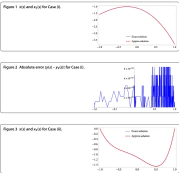
Figure 1 x(s) andx5(s) for Case (i).

Figure 2 Absolute error|y(s) –y5(s)|for Case (i).

Figure 3 x(s) andx5(s) for Case (ii).

Example ([, ]) Let us consider the ﬁrst kind of Cauchy type singular Fredholm

in-tegral equation given by



–

y(t)

t–sdt=g(s), – <s< , ()

whereg(s) =s_{+ }_s_{+ }_s₊_s_– .

This equation has an exact solution for all following cases:

Case (i) : y(s) = –

π

√  –s

s+ s+ s+

 

,

Case (ii) : y(s) = 

π√ –s

s+ s+ 

s–s– s–

 

,

Case (iii) : y(s) = –

π

 –s

 +s

s+ s+  s

_{+ }_s₊ 

,

Case (iv) : y(s) = 

π

 +s

 –s

s+ s– s

₊_s_– 

.

(12)

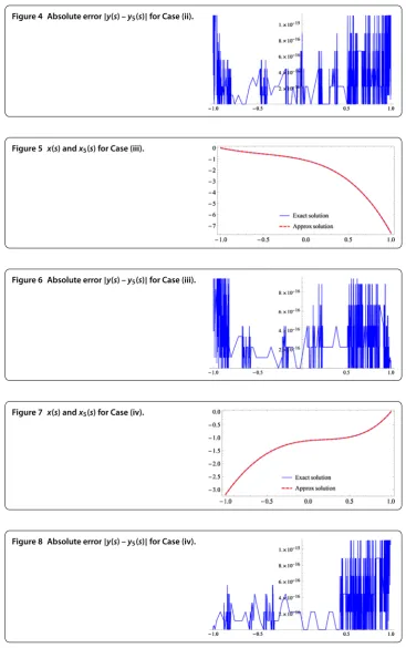
Figure 4 Absolute error|y(s) –y5(s)|for Case (ii).

Figure 5 x(s) andx5(s) for Case (iii).

Figure 6 Absolute error|y(s) –y5(s)|for Case (iii).

Figure 7 x(s) andx5(s) for Case (iv).

Figure 8 Absolute error|y(s) –y5(s)|for Case (iv).

(13)

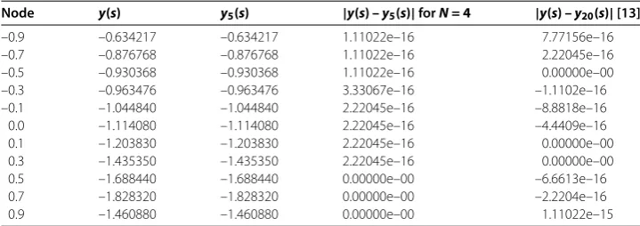
Table 1 Numerical results of Example 1 for Case (i)

Node y(s) y5(s) |y(s) – y5(s)|forN = 4 |y(s) – y20(s)|[13]

–0.9 –0.634217 –0.634217 2.22045e–16 3.33067e–16

–0.7 –0.876768 –0.876768 0.00000e–00 1.77636e–15

–0.5 –0.930368 –0.930368 1.11022e–16 –5.5511e–16

–0.3 –0.963476 –0.963476 2.22045e–16 2.22045e–16

–0.1 –1.044840 –1.044840 2.22045e–16 2.22045e–16

0.0 –1.114080 –1.114080 0.00000e–00 6.66134e–16

0.1 –1.203830 –1.203830 0.00000e–00 0.00000e–00

0.3 –1.435350 –1.435350 2.22045e–16 6.66134e–16

0.5 –1.688440 –1.688440 0.00000e–00 8.88179e–16

0.7 –1.828320 –1.828320 2.22045e–16 0.00000e–00

0.9 –1.460880 –1.460880 4.44089e–16 2.22045e–16

Table 2 Numerical results of Example 1 for Case (ii)

–0.9 –0.634217 –0.634217 1.11022e–16 –6.6613e–16

–0.7 –0.876768 –0.876768 1.11022e–16 7.49401e–16

–0.5 –0.930368 –0.930368 1.11022e–16 –5.5511e–16

–0.3 –0.963476 –0.963476 2.22045e–16 4.16334e–16

–0.1 –1.044840 –1.044840 2.22045e–16 –3.3307e–16

0.0 –1.114080 –1.114080 2.22045e–16 1.66533e–16

0.1 –1.203830 –1.203830 0.00000e–00 5.55112e–16

0.3 –1.435350 –1.435350 2.22045e–16 0.00000e–00

0.5 –1.688440 –1.688440 0.00000e–00 –7.7716e–16

0.7 –1.828320 –1.828320 0.00000e–00 0.00000e–00

0.9 –1.460880 –1.460880 2.22045e–16 9.43690e–16

Table 3 Numerical results of Example 1 for Case (iii)

–0.9 –0.634217 –0.634217 2.22045e–16 3.21965e–15

–0.7 –0.876768 –0.876768 4.44089e–16 3.33067e–16

–0.5 –0.930368 –0.930368 1.11022e–16 –2.2204e–16

–0.3 –0.963476 –0.963476 2.22045e–16 1.44329e–15

–0.1 –1.044840 –1.044840 0.00000e–00 6.66134e–16

0.0 –1.114080 –1.114080 2.22045e–16 6.66134e–16

0.1 –1.203830 –1.203830 2.22045e–16 2.22045e–16

0.3 –1.435350 –1.435350 2.22045e–16 2.22045e–16

0.5 –1.688440 –1.688440 2.22045e–16 4.44090e–16

0.7 –1.828320 –1.828320 0.00000e–00 4.44090e–16

0.9 –1.460880 –1.460880 4.44089e–16 –8.8818e–16

Table 4 Numerical results of Example 1 for Case (iv)

–0.9 –0.634217 –0.634217 1.11022e–16 7.77156e–16

–0.7 –0.876768 –0.876768 1.11022e–16 2.22045e–16

–0.5 –0.930368 –0.930368 1.11022e–16 0.00000e–00

–0.3 –0.963476 –0.963476 3.33067e–16 –1.1102e–16

–0.1 –1.044840 –1.044840 2.22045e–16 –8.8818e–16

0.0 –1.114080 –1.114080 2.22045e–16 –4.4409e–16

0.1 –1.203830 –1.203830 2.22045e–16 0.00000e–00

0.3 –1.435350 –1.435350 2.22045e–16 0.00000e–00

0.5 –1.688440 –1.688440 0.00000e–00 –6.6613e–16

0.7 –1.828320 –1.828320 0.00000e–00 –2.2204e–16

(14)

Figure 9 x(s) andx5(s) for Case (i).

Figure 10 Absolute error|y(s) –y5(s)|for Case (i).

Figure 11 x(s) andx5(s) for Case (ii).

Figure 12 Absolute error|y(s) –y5(s)|for Case (ii).

Example  Suppose we have the following CSFIE:



–

y(t)

t–sdt=g(s), – <s< , ()

whereg(s) = –s₊ s–

(15)

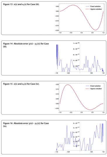
Figure 13 x(s) andx5(s) for Case (iii).

Figure 14 Absolute error|y(s) –y5(s)|for Case (iii).

Figure 15 x(s) andx5(s) for Case (iv).

Figure 16 Absolute error|y(s) –y5(s)|for Case (iv).

This equation has exact solution for all following cases:

Case (i) : y(s) = –

π

√

 –s_–_s₊_s_, Case (ii) : y(s) = 

π√ –s

–s+ s–s,

Case (iii) : y(s) = –

π

 –s

 +s

(16)

Table 5 Numerical results of Example 2 for Case (i)

Node y(s) y5(s) |y(s) – y5(s)|

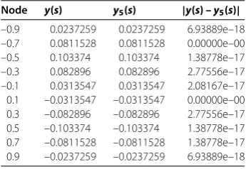
–0.9 0.0237259 0.0237259 6.93889e–18 –0.7 0.0811528 0.0811528 0.00000e–00 –0.5 0.103374 0.103374 1.38778e–17 –0.3 0.082896 0.082896 2.77556e–17 –0.1 0.0313547 0.0313547 2.08167e–17 0.1 –0.0313547 –0.0313547 0.00000e–00 0.3 –0.082896 –0.082896 2.77556e–17 0.5 –0.103374 –0.103374 1.38778e–17 0.7 –0.0811528 –0.0811528 1.38778e–17 0.9 –0.0237259 –0.0237259 6.93889e–18

Table 6 Numerical results of Example 2 for Case (ii)

Node y(s) y5(s) |y(s) – y5(s)|

–0.9 0.0237259 0.0237259 2.77556e–17 –0.7 0.0811528 0.0811528 1.38778e–17 –0.5 0.103374 0.103374 1.38778e–17 –0.3 0.082896 0.082896 1.38778e–17 –0.1 0.0313547 0.0313547 2.08167e–17 0.1 –0.0313547 –0.0313547 3.46945e–17 0.3 –0.082896 –0.082896 4.16334e–17 0.5 –0.103374 –0.103374 1.38778e–17 0.7 –0.0811528 –0.0811528 1.38778e–17 0.9 –0.0237259 –0.0237259 7.63278e–17

Table 7 Numerical results of Example 1 for Case (iii)

Node y(s) y5(s) |y(s) – y5(s)|

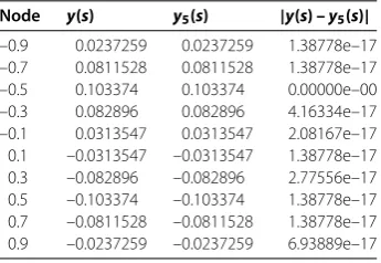
–0.9 0.0237259 0.0237259 2.08167e–17 –0.7 0.0811528 0.0811528 1.38778e–17 –0.5 0.103374 0.103374 1.38778e–17 –0.3 0.082896 0.082896 2.77556e–17 –0.1 0.0313547 0.0313547 2.08167e–17 0.1 –0.0313547 –0.0313547 6.93889e–18 0.3 –0.082896 –0.082896 2.77556e–17 0.5 –0.103374 –0.103374 0.00000e–00 0.7 –0.0811528 –0.0811528 0.00000e–00 0.9 –0.0237259 –0.0237259 3.46945e–18

Case (iv) : y(s) = 

π

 +s

 –s

–s+s+s–s.

In Figures , ,  and , we plot the exact solutions and the approximate solutions forn=  andN=  for all cases and it is clear that the approximate solution is in good agreement with the exact solution. Also, the errors of the presented method are plotted in Figures , ,  and  and are presented in all cases in Tables , ,  and .

7 Conclusion

(17)

Table 8 Numerical results of Example 1 for Case (iv)

Node y(s) y5(s) |y(s) – y5(s)|

–0.9 0.0237259 0.0237259 1.38778e–17 –0.7 0.0811528 0.0811528 1.38778e–17 –0.5 0.103374 0.103374 0.00000e–00 –0.3 0.082896 0.082896 4.16334e–17 –0.1 0.0313547 0.0313547 2.08167e–17 0.1 –0.0313547 –0.0313547 1.38778e–17 0.3 –0.082896 –0.082896 2.77556e–17 0.5 –0.103374 –0.103374 1.38778e–17 0.7 –0.0811528 –0.0811528 1.38778e–17 0.9 –0.0237259 –0.0237259 6.93889e–17

equations in all cases has been set and an approximation for the integral in determining the system of linear equations was implemented as well. By comparing the approximate solutions with the exact solutions in the numerical results, it is obvious that the approxi-mate solutions are close to the well-known results for various cases.

Competing interests

The authors declare that they have no competing interests.

Authors’ contributions

All authors read and approved the ﬁnal manuscript.

Publisher’s Note

Springer Nature remains neutral with regard to jurisdictional claims in published maps and institutional aﬃliations.

Received: 6 April 2017 Accepted: 26 August 2017 References

1. Erdogan, F, Gupta, GD, Cook, TS: Numerical solution of singular integral equations. In: Sih, GC (ed.) Methods of Analysis and Solutions of Crack Problems: Recent Developments in Fracture Mechanics Theory and Methods of Solving Crack Problems, pp. 368-425. Springer, Dordrecht (1973)

2. Ladopoulos, E: Singular Integral Equations: Linear and Non-linear Theory and Its Applications in Science and Engineering. Springer, New York (2013)

3. Gakhov, F: Boundary Value Problems. Dover, New York (1990)

4. Kim, S: Solving singular integral equations using Gaussian quadrature and overdetermined system. Comput. Math. Appl.35(10), 63-71 (1998)

5. Golberg, M: Introduction to the numerical solution of Cauchy singular integral equations. In: Numerical Solution of Integral Equations, pp. 183-308. Springer, Berlin (1990)

6. Lifanov, IK: Singular Integral Equations and Discrete Vortices. Vsp, Utrecht (1996)

7. Jen, E, Srivastav, R: Cubic splines and approximate solution of singular integral equations. Math. Comput.37(156), 417-423 (1981)

8. Kim, S: Numerical solutions of Cauchy singular integral equations using generalized inverses. Comput. Math. Appl.

38(5), 183-195 (1999)

9. Mennouni, A, Guedjiba, S: A note on solving Cauchy integral equations of the ﬁrst kind by iterations. Appl. Math. Comput.217(18), 7442-7447 (2011)

10. Mandal, B, Bhattacharya, S: Numerical solution of some classes of integral equations using Bernstein polynomials. Appl. Math. Comput.190(2), 1707-1716 (2007)

11. Karczmarek, P, Pylak, D, Sheshko, MA: Application of Jacobi polynomials to approximate solution of a singular integral equation with Cauchy kernel. Appl. Math. Comput.181(1), 694-707 (2006)

12. Yaghobifar, M, Long, NN, Eshkuvatov, Z: Analytical solutions of characteristic singular integral equations in the class of rational functions. Int. J. Contemp. Math. Sci.5(56), 2773-2779 (2010)

13. Eshkuvatov, Z, Long, NN, Abdulkawi, M: Approximate solution of singular integral equations of the ﬁrst kind with Cauchy kernel. Appl. Math. Lett.22(5), 651-657 (2009)

14. De Bonis, MC, Laurita, C: Nyström method for Cauchy singular integral equations with negative index. J. Comput. Appl. Math.232(2), 523-538 (2009)

15. Liu, D, Zhang, X, Wu, J: A collocation scheme for a certain Cauchy singular integral equation based on the superconvergence analysis. Appl. Math. Comput.219(10), 5198-5209 (2013)

16. Panja, M, Mandal, B: Solution of second kind integral equation with Cauchy type kernel using Daubechies scale function. J. Comput. Appl. Math.241, 130-142 (2013)

(18)

18. Setia, A, Sharma, V, Liu, Y: Numerical solution of Cauchy singular integral equation with an application to a crack problem. Neural Parallel Sci. Comput.23, 387-392 (2015)

19. Abdulkawi, M: Solution of Cauchy type singular integral equations of the ﬁrst kind by using diﬀerential transform method. Appl. Math. Model.39(8), 2107-2118 (2015)

20. Beyrami, H, Lotﬁ, T, Mahdiani, K: A new eﬃcient method with error analysis for solving the second kind Fredholm integral equation with Cauchy kernel. J. Comput. Appl. Math.300, 385-399 (2016)

21. Dezhbord, A, Lotfi, T, Mahdiani, K: A new efficient method for cases of the singular integral equation of the first kind. J. Comput. Appl. Math.296, 156-169 (2016)

22. Yüzba¸sı, ¸S, Sezer, M: A numerical method to solve a class of linear integro-diﬀerential equations with weakly singular kernel. Math. Methods Appl. Sci.35(6), 621-632 (2012)

23. Yüzba¸sı, ¸S, Karaçayır, M: A Galerkin-like approach to solve high-order integrodiﬀerential equations with weakly singular kernel. Kuwait J. Sci.43(2) 106-120 (2016)

24. I¸sik, OR, Sezer, M, Güney, Z: Bernstein series solution of a class of linear integro-diﬀerential equations with weakly singular kernel. Appl. Math. Comput.217(16), 7009-7020 (2011)

25. Youseﬁ, S, Behroozifar, M, Dehghan, M: Numerical solution of the nonlinear age-structured population models by using the operational matrices of Bernstein polynomials. Appl. Math. Model.36(3), 945-963 (2012)

26. Yuzbasi, S: A collocation method based on Bernstein polynomials to solve nonlinear Fredholm-Volterra integro-diﬀerential equations. Appl. Math. Comput.273, 142-154 (2016). doi:10.1016/j.amc.2015.09.091 27. Yüzba¸sı, ¸S: Numerical solutions of fractional Riccati type diﬀerential equations by means of the Bernstein