Exponentially practical stability of discrete time singular system with delay and disturbance

(1)

R E S E A R C H

Open Access

Exponentially practical stability of discrete

time singular system with delay and

disturbance

S. Wangrat

1

_{and P. Niamsup}

1,2*

*_{Correspondence:}

[email protected]

1_{Department of Mathematics,}

Chiang Mai University, Chiang Mai, Thailand

2_{Centre of Excellence in}

Mathematics, CHE, Bangkok, Thailand

Abstract

In this paper, we consider exponentially practical stability of a discrete time singular system with disturbance. By using Lyapunov–Krasovskii stability theory, some criteria for exponentially practical stability of such a system are derived. Moreover, by using a Razumikhin-type technique, the criteria for exponentially practical stability of a discrete time singular system with delay and disturbance are also obtained. Some numerical examples are given to show the success of our theoretical results.

Keywords: Discrete time system; Singular system; Delay; Exponentially practical stability; Disturbance

1 Introduction

Singular systems, which are also called descriptor systems, implicit systems, or general-ized systems, have been investigated extensively in many areas [1–21]. Generally, the sys-tems can be described using algebraic and diﬀerential equations. Such syssys-tems are natural presentations of several dynamic systems which are better than regular systems, such as economical systems, chemical systems, robotic systems, etc. [1–10, 12–14, 20–22]. More-over, singular systems are very complicated because we have to consider the stability of the systems as well as the regularity and also impulse free (in case of continuous singular sys-tems) or causality (in case of discrete singular syssys-tems) [2, 11, 18]. In addition, a discrete time system is often represented in the real world systems such as population models and switched systems. There are several studies on the stability of a discrete time system [2–4, 8–15, 17, 18, 22–24].

In real world systems, the variation of systems’ current status often depends not only on the current state but also on the past state of the systems; such systems are called time delay systems. Examples of time delay systems are population dynamic models, mechani-cal transmissions, and digital control systems [4, 7–10, 12–14]. It is well known that time delay may cause instability, oscillation, and poor performance of systems. For the above-mentioned reasons, time delay systems have been extensively discussed in many litera-ture works [2, 4, 6–10, 13–16, 18, 19, 22, 23]. As is known, most common approaches to studying stability analysis of a time delay system are Lyapunov–Krasovskii functional ap-proach and Razumikhin-type technique. In the case of Lyapunov–Krasovskii functional method, it requires that a candidate Lyapunov–Krasovskii functional is decreasing on the

(2)

whole state space. Meanwhile, the Razumikhin-type technique has an advantage that the Lyapunov–Krasovskii functional is not required to be decreasing on the whole state space. In general, disturbance inputs often occur in modeling of phenomena and engineering sys-tems which may be due to data transformation, unknown disturbances, or measurement errors [4, 10, 24, 25]. Therefore, it is important to study the stability of a discrete time singular system with delay and disturbance.

Considering asymptotic stability, it is more desirable to consider exponential stability criterion for dynamical systems [1, 6–10, 18–21, 24, 25]. For exponential stability, it is re-quired that all solutions starting near an equilibrium point not only stay nearby, but tend to the equilibrium point very fast with exponential decay rate. In practice, we may only need to stabilize a system into the region of a phase space where the system may oscillate near the state in which the implementation is still acceptable. This concept is called prac-tical stability [18, 22, 26–29] which is very useful for studying the asymptotic behavior of the system in which the origin is not necessarily an equilibrium point. In this case, practi-cal stability is an important concept to analyze the asymptotic behavior of solutions with respect to a small neighborhood of the origin. Recently, there have been several studies on practical stability of continuous time systems with delay, see [26–29]. However, there have been few studies on practical stability of discrete time systems with delay [22, 23]. In [3], the authors studied discrete time singular systems with disturbance and obtained some stability criteria by using Lyapunov stability theory. In [23], the authors used the Razumikhin-type technique to derive the exponentially practical stability condition for impulsive discrete time systems with delay. Motivated by the above discussions, we pro-pose to study exponentially practical stability of a discrete time singular system with delay and disturbance. We shall derive a new criterion for exponentially practical stability of the system, namely the solutions tend to the origin state with exponential decay rate in the early stage (but eventually oscillate in a neighborhood of the origin), in which the perfor-mance is still acceptable.

This work is organized as follows. In Sect. 2, some notations and definitions are intro-duced. In Sect. 3, we present some criteria for exponentially practical stability of a discrete time system with disturbance, exponentially practical stability of a discrete time singular system with disturbance, exponentially practical stability of a discrete time system with delay and disturbance, and exponentially practical stability of a discrete time singular sys-tem with delay and disturbance; definitions and assumption will be used in the proof our result. Some numerical examples are given to show the effectiveness of our theoretical result in Sect. 4. The last section concludes the work.

2 Preliminaries

Consider the following discrete time singular system with delay and disturbance:

⎧ ⎨ ⎩

Ex(k+ 1) =Ax(k) +Bx(k–τ) +Gw(k),

x(s) =ϕ(s), s∈Nk0–τ,

(2.1)

wherex(k)∈Rn_{is the state vector,}_w₍_k₎_∈₌_{_w₍_k₎_∈_Rm_/_w₍_k₎_≤_w_,_∃_w_{> 0,}_∀_k_≥_k 0}

is the disturbance, A,B,G, and E are constant matrices with appropriate dimensions where E is a singular matrix withrank(E) =r<n, τ is constant delay, ϕ∈ Cτ :={f :

(3)

Nk0–τ ={k0–τ,k0–τ+ 1, . . . ,k0– 1,k0}, andNk0={k0,k0+ 1,k0+ 2, . . .},k0≥0. A function

ρ:R+

0−→R, is called aK-function if it is a nonnegative continuous function whereR+0is

the set of nonnegative real numbers. Let ﬂoor(r) := rbe the greatest integer that is less than or equal tor, and let ceil(r) :=rbe the least integer that is greater than or equal tor.

Deﬁnition 2.1([18]) System (2.1) is said to beregularifdet(zE–A)= 0 for somez∈C. System (2.1) is said to becausalifdeg(det(zE–A)) =rank(E).

3 Main results

In this section, we consider exponentially practical stability problems for the following four cases: a discrete time system with disturbance, a discrete time singular system with disturbance, a discrete time system with delay and disturbance, and a discrete time singu-lar system with delay and disturbance.

First, we consider the discrete time system with disturbance as follows:

⎧ ⎨ ⎩

x(k+ 1) =f(k,x(k),w(k)),

x(k0) =x0,

(3.1)

where disturbance w(k)∈, where is deﬁned as in (2.1),f :R×Rn_×_−→_Rn_is

continuous and locally Lipschitz in (x,w), uniformly inkwith Lipschitz constantLwhich satisﬁes f(k, 0, 0) = 0. Letx(k;k0,x0,w) denote the trajectory of system (3.1) with initial statex(k0) =x0and disturbance signalw(k)∈.

Deﬁnition 3.1 System (3.1) is exponentially practically stable in the pth-moment for

somep> 0 if for allk≥k0there exist constants 0 <λ< 1,η> 0,r> 0 such that

x(k;k0,x0,w)p≤ηx0pλk–k0₊_r_, ∀_w₍_k₎∈_.

Theorem 3.1 If there exist a Lyapunov function V(k,x(k)),a K -functionρ,and positive constants c1,c2,c3,a,p;c3<c2such that the following conditions hold for all k≥k0,x(k)∈

Rn_,_w₍_k₎_∈_:

(i) c1x(k)p_≤_V₍_k_,_x₍_k₎₎_≤_c2_x₍_k₎p₊_a_,

(ii) V(k,x(k)) =V(k+ 1,x(k+ 1)) –V(k,x(k))≤–c3x(k)p₊_ρ₍_w₍_k₎₎_.

Then system(3.1)is exponentially practically stable in the pth-moment withη=c2 c1,λ=

1 –c3

c2,and r= a c1 +

a1

c1(1–σ),where a1= c3a

c2 +ρ1andρ1=supw(k)∈{ρ(w(k))}.

Proof From (i) and (ii), we obtain that

Vk+ 1,x(k+ 1;k0,x0,w)–Vk,x(k;k0,x0,w)

≤–c3x(k;k0,x0,w)p+ρw(k)

≤–c3

c2

Vk,x(k;k0,x0,w)+c3a

c2

+ρ1

= –c3

c2V

(4)

for allk≥k0,w(k)∈, whereρ1=supw(k)∈{ρ(w(k))},a1=

c3a

c2 +ρ1. Without loss of

generality, we may assume thatc3<c2, and letσ= 1 –c3

c2. Then 0 <σ< 1, and it follows

that

Vk+ 1,x(k+ 1;k0,x0,w)

≤

1 –c3

c2 V

k,x(k;k0,x0,w)+a1

=σVk,x(k;k0,x0,w)+a1

≤σσVk– 1,x(k– 1;k0,x0,w)+a1+a1

≤σ2σVk– 2,x(k– 2;k0,x0,w)+a1+σa1+a1

.. .

≤σk+1V(k0,x0,w) +σka1+σk–1a1+· · ·+a1.

Thus,

Vk,x(k;k0,x0,w)≤σk–k0_V₍_k0_,_x0_,_w_{) +} a1

1 –σ.

From (i), we can see that

c1x(k;k0,x0,w)p≤Vk,x(k;k0,x0,w)≤σk–k0_V₍_k0_,_x0_,_w_{) +} a1

1 –σ

≤σk–k0_c2_x0p₊_a₊ a1

1 –σ.

Thus,

x(k;k0,x0,w) p

≤c2

c1σ k–k0_x

0p+

σk–k0_a c1 +

a1 c1(1 –σ)

≤c2

c1

σk–k0_x0p₊ a c1

+ a1

c1(1 –σ)

=c4σk–k0x0p+a2,

wherec4=c2

c1 anda2= a c1 +

a1

c1(1–σ). It follows that

x(k;k0,x0,w)p≤c4σk–k0_x0p₊_a2 _{for all}_k≥_k0_,_w₍_k₎∈_.

Therefore, system (3.1) is exponentially practically stable in the pth-moment withη=

c4,λ=σ, andr=a2.

Then, we will consider system (2.1) without delay, namely a discrete time singular system with disturbance, as follows:

⎧ ⎨ ⎩

Ex(k+ 1) =Ax(k) +Gw(k),

x(k0) =x0.

(5)

Deﬁnition 3.2 The singular system (3.2) is said to be exponentially practically stable in thepth-moment for somep> 0 if, for allk≥k0, there exist constants 0 <λ< 1,η> 0,r> 0 for each disturbancew(k)∈such that

Ex(k;k0,x0,w)p≤ηx0pλk–k0₊_r_,

wherex(k,k0,x0,w) is the state trajectory of a system with initial statex0.

Theorem 3.2 Assume that the singular system(3.2)is regular and causal.Then the

singu-lar system(3.2)is exponentially practically stable in the pth-moment with respect to w(k),

if there exists a Lyapunov function V(k,x(k))such that

(i) c1Ex(k)p_≤_V₍_k_,_x₍_k₎₎_≤_c2_Ex₍_k₎p₊_a_,

(ii) V(k,x(k)) =V(k+ 1,x(k+ 1)) –V(k,x(k))≤–c3x(k)p₊_ρ₍_w₍_k₎₎_{hold for some} positive constantsa,c1,c2,c3,p;c3<c2and aK-functionρ.

Proof Assume that system (3.2) is regular and causal. Then, from [30], there exist nonsin-gular matricesM,Nwith appropriate dimensions such that

MEN=

, then system (3.2) is transformed to the system

y1(k+ 1) =A1y1(k) +G1w(k), (3.3)

y2(k) = –G2w(k) (3.4)

with initial statey0satisfyingIr0

0 0 isfying conditions (i) and (ii), we obtain the following estimations:

(6)

From which it follows that

Vk,y1(k)≥c1M–1N–1y1(k)2 p

2

=c1y1T(k)M–1N–1TM–1N–1y1(k) p

2

≥c1

λmin

M–1N–1TM–1N–1

p

2_y 1(k)

p

.

Similarly, we have

Vk,y1(k)≤c2M–1pN–1py1(k)p+a.

Thus,

c1y1(k)p≤Vk,y1(k)≤c2y1(k)p+a,

wherec1=c1(λmin((M–1N–1)T(M–1N–1)))

p

2, andc₂=c₂M–1pN–1p.

Furthermore, we have the following estimations for V(k,x(k)):

Vk,x(k)=Vk+ 1,x(k+ 1)–Vk,x(k)≤–c3x(k)p+ρw(k),

Vk,Ny(k)=Vk+ 1,Ny(k+ 1)–Vk,Ny(k)≤–c3Ny(k)p+ρw(k),

Vk,y(k)=Vk+ 1,y(k+ 1)–Vk,y(k)≤–c3y(k)p+ρw(k),

Vk,y1(k)=Vk+ 1,y1(k+ 1)–Vk,y1(k)≤–c3y1(k)p+ρw(k).

From (3.3) withy1(k) =Ny1(k) 0

, we have

y1(k+ 1) =A1y1(k) +G1w(k), (3.5)

whereA1=N _A₁ ₀

0 0

N–1_,_G 1=N

_G₁₀ 0 0

, andw(k) =w(k)

0

. Therefore, we may conclude that there exists a Lyapunov functionV(k,y1(k)) for system (3.5) which satisﬁes the following

conditions:

(i) c1y1(k)p_≤_V₍_k_,_y1₍_k₎₎_≤_c2_y1₍_k₎p₊_a_,

(ii) V(k,y1(k)) =V(k+ 1,y1(k+ 1)) –V(k,y1(k))≤–c3y1(k)p+ρ(w(k)). Hence, from Theorem 3.1, there exist constants 0 <λ< 1,η0> 0,r0> 0 such that

y1(k)p≤η0y10pλk–k0+r0, ∀k≥k0, (3.6)

wherey10=Ny10 0

. Thus, we have

y1(k) p

≤η0N–1 p

Npy10pλk–k0+N–1 p

r0

=η1y10pλk–k0+r1, ∀k≥k0, (3.7)

whereη1=η0N–1pNp,r1=N–1pr0. From (3.4), we havey2(k) = –G2w(k), which in

turn gives

(7)

Thus, it follows from (3.7) and (3.8) that

From (3.9), there are four cases to be considered according to the values ofpandr1as

(8)

(9)

whereη4=η 1

n

1y10

p

n–p_,_r5₌_r1₊_w_G2_{, and 0 <}_λ₁₌_λn1 _{< 1. Therefore, from (}_Case_{I) to}

(CaseIV), we obtain

y(k)≤η5y10pλk2–k0+r6, (3.10)

whereη5=max{η2,η3,η4},r6=max{r2,r3,r4,r5}, and 0 <λ2=min{λ,λ1}< 1.

FromMEx0=MENy0=Ir 0

0 0

y0andy0=y10 0

, it follows thaty10 ≤ MEx0. Sincex(k) =Ny(k), it follows from (3.10) that

Ex(k)≤ ENy(k)

≤ ENη5y10pλk2–k0+r6

≤η5ENMpEpx0pλk2–k0+ENr6

=η6x0λk2–k0+r7,

whereη6=η5Ep+1NMpx0p–1andr7=ENr6.

Therefore, the singular system (3.2) is exponentially practically stable with respect to

w(k) withη=η6,λ=λ2, andr=r7.

Remark3.1 In Theorem 3.2, forp= 1, we can show that the singular system (3.2) is ex-ponentially practically stable in thepth-moment with respect tow(k) by considering the explicit form of solution of the system. System (3.2) may be reduced to system (3.3) and (3.4). Moreover, the explicit solution of (3.3) and (3.4) withk0= 0 is given as follows:

y1(k) =Ak1y1(0) + k–1

i=0

Ak₁–1–iG1w(i), (3.11)

y2(k) = –G2w(k). (3.12)

Thus, from (3.11) and (3.12), we have

y(k)≤y1(k)+y2(k)

≤ A1ky1(0)+ k–1

i=0

A1k–1–iG1w(i)+G2w(k).

By assuming thatA1< 1, we obtain

y(k)≤ A1ky1(0)+wG1

1

1 –A1+wG2

=A1ky1(0)+r0,

wherer0=wG1_1–1_A₁+wG2. Sincex(k) =Ny(k), we have that

_Ex₍_k₎_≤_E_N_y₍_k₎

(10)

≤ ENA1kMEx(0)+r0

=ηx(0)A1k+r,

whereη=E2_N_M_and_r₌_E_N_r0_{. Hence, system (3.2) is exponentially}

practi-cally stable.

Next, we consider the discrete time system with delay and disturbance as follows:

⎧ ⎨ ⎩

x(k+ 1) =f(k,xk,w(k)),

x(s) =ϕ(s), s∈Nk0–τ,

(3.13)

wherexkis deﬁned byxk(s) =x(k+s) for anys∈Nk0–τ, disturbancew(k)∈, whereis

deﬁned as in (2.1),f:R×Rn_×_−→_Rn_{is continuous and locally Lipschitz in (}_x_,_w_),

uni-formly inkwith Lipschitz constantLwhich satisﬁesf(k, 0, 0) = 0. Letx(k;k0,ϕ,w) denote the trajectory of system (3.13) with initial conditionϕand disturbance signalw(k)∈.

Deﬁnition 3.3 System (3.13) is exponentially practically stable in thepth-moment with

respect tow(k) for somep> 0 if, for anyk≥k0, there exist constants 0 <λ< 1,η> 0,r> 0 such that

x(k;k0,φ,w)p≤ηϕpλk–k0₊_r_, ∀_w₍_k₎∈_.

Theorem 3.3 If there exist a Lyapunov–Krasovskii functional V(k,x(k)),a K -functionρ,

and positive constants c1,c2,a,p,q,β,where q> 1, 0 <β< 1,ρ(w(k)) <βa such that the following conditions hold for all w(k)∈:

(i) c1x(k)p_≤_V₍_k_,_x₍_k₎₎_≤_c2_x₍_k₎p₊_a_,

(ii) IfV(k+s,x(k+s))≤qV(k+ 1,x(k+ 1))withs∈Nk0–τ,then

Vk,x(k)=Vk+ 1,x(k+ 1)–Vk,x(k)≤–βVk,x(k)+ρw(k).

Then system(3.13)is exponentially practically stable in thepth-moment with

η=c2 c1,q

–_τ1₊₁_≤_λ_{< 1}_,_and_r₌ a c1.

Proof Forq> 1, there exists 0 <λ< 1 such thatq≥λ–(τ+1), or equivalently,q–_τ1₊₁_≤_λ_{< 1.}

By employing a similar approach as in the proof of Theorem (3.1) in [23], it follows from 0 <β< 1 andρ(w(k)) <βathat

Vk,x(k)≤c2ϕpλk–k0₊_a

fork≥k0,w(k)∈, from which it follows that

x(k)p≤c2

c1ϕ

p_λk–k0₊ a

c1, k≥k0,w(k)∈.

Therefore, system (3.13) is exponentially practically stable in thepth-moment withη=

c2 c1,q

–_τ1₊₁_≤_λ_{< 1, and}_r₌ a

(11)

Finally, we consider exponentially practical stability for system (2.1) with delay and dis-turbance.

Deﬁnition 3.4 The discrete time singular system (2.1) is said to be exponentially

practi-cally stable in thepth-moment for somep> 0 if there exist constants 0 <λ< 1,η> 0,r> 0 for each disturbancew(k)∈such that

Ex(k;k0,ϕ,w) p

≤ηϕpλk–k0₊_r

for allk≥k0, wherex(k;k0,ϕ,w) is the state trajectory of the system with initial condition ϕ. In particular, whenp= 2, the system is said to be exponentially practically stable in the mean square.

In order to proceed with the main result on exponentially practical stability in thep th-moment of a singular system with delay and disturbance (2.1), we make the following as-sumption; an explanation for this assumption is given in Remark 3.2.

Assumption 3.1 There exist nonsingular matrices M,N with appropriate dimensions

such that MEN =Ir 0

0 0n–r

, MAN =A1 0

0 In–r

, MBN =B1 0

B3B4

, and MG=G1

G2

, where B4< 1.

Remark3.2 For a physical meaning of Assumption 3.1, it implies that there is a plant (y1) in this situation which does not dynamically depend on the other plant (y2). For future

investigation, we propose to study a more general case in whichMBN=B1B2 B3B4

, whereB2

may not be zero; namely, all plants dynamically interact, and thatB4may not be less than 1.

Theorem 3.4 Assume that the singular system(2.1)is regular and causal,and that

As-sumption3.1holds.Then the singular system(2.1)is exponentially practically stable in the pth-moment with respect to w(k), if there exists a Lyapunov–Krasovskii functional V(k,x(k))such that

(i) c1Ex(k)p_≤_V₍_k_,_x₍_k₎₎_≤_c2_Ex₍_k₎p₊_a_,

(ii) IfV(k+s,x(k+s))≤qV(k+ 1,x(k+ 1))withs∈Nk0–τ,then

Vk,x(k)=Vk+ 1,x(k+ 1)–Vk,x(k)≤–βVk,x(k)+ρw(k)

hold for some positive constantsa,c1,c2,p,q,β,whereq> 1, 0 <β< 1,and some K-functionρ.

Proof Assume that system (2.1) is regular and causal. Then, from [30] and Assumption 3.1, there exist nonsingular matricesM,Nsuch that

MEN=

Ir 0

0 0n–r

, MAN=

A1 0

0 In–r

,

MBN=

B1 0 B3 B4

, MG=

G1 G2

(12)

whereB4< 1. Lety(k) =N–1_x₍_k_{) =}y1(k) y2(k)

, then system (2.1) is transformed to the fol-lowing system:

y1(k+ 1) =A1y1(k) +B1y1(k–τ) +G1w(k), (3.14)

y2(k) = –B3y1(k–τ) –B4y2(k–τ) –G2w(k), (3.15)

y1(s) :=φ1(s) =N–1ϕ1(s), s∈Nk0–τ,

y2(s) :=φ2(s) =N–1ϕ2(s), s∈Nk0–τ.

From the assumption, there exists a Lyapunov–Krasovskii functionalV(k,x(k)) which sat-isﬁes conditions (i) and (ii). Then we obtain the following estimations:

(13)

Now, assume that the following inequalities hold:

Vk+s,x(k+s)≤qVk+ 1,x(k+ 1) withs∈Nk0–τ,

Vk+s,Ny(k+s)≤qVk+ 1,Ny(k+ 1) withs∈Nk0–τ,

Vk+s,y(k+s)≤qVk+ 1,y(k+ 1) withs∈Nk0–τ, Vk+s,y1(k+s)

≤qVk+ 1,y1(k+ 1)

withs∈Nk0–τ.

Then it follows from (ii) that

Vk,x(k)=Vk+ 1,x(k+ 1)–Vk,x(k)≤–βVk,x(k)+ρw(k),

Vk,Ny(k)=Vk+ 1,Ny(k+ 1)–Vk,Ny(k)≤–βVk,Ny(k)+ρw(k),

Vk,y(k)=Vk+ 1,y(k+ 1)–Vk,y(k)≤–βVk,y(k)+ρw(k),

Vk,y1(k)=Vk+ 1,y1(k+ 1)–Vk,y1(k)≤–βVk,y1(k)+ρw(k).

Sincey1(k) =Ny1(k) 0

, it follows from (3.14) that

y1(k+ 1) =A1y1(k) +B1y1(k–τ) +G1w(k), (3.16)

whereA1=NA10 0 0

N–1_,_B1₌_NB10 0 0

N–1_,_G1₌_NG10 0 0

, andw(k) =w₀(k). Therefore, we may conclude that there exists a Lyapunov–Krasovskii functionalV(k,y1(k)) for system (3.16) which satisﬁes the following conditions:

(i) c1¯y1(k)p≤V(k,y1(k))≤ ¯c2y1(k)p+a,

(ii) IfV(k+s,y1(k+s))≤qV(k+ 1,y1(k+ 1))withs∈Nk0–τ, then

Vk,y1(k)=Vk+ 1,y1(k+ 1)–Vk,y1(k)≤–βVk,y1(k)+ρw(k).

Thus, from Theorem 3.3, there exist constants 0 <λ< 1,η0≥0,r0> 0 such that

y1(k) p

≤η0φ1pλk–k0+r0, ∀k≥k0, (3.17)

whereφ₁=Nφ1 0

. It follows that

y1(k) p

≤η0N–1 p

Npφ1pλk–k0+N–1 p

r0

=η1φ1pλk–k0+r1, ∀k≥k0, (3.18)

whereη1=η0N–1pNp,r1=N–1pr0. Therefore, we obtain

y1(k)≤η1φ1pλk–k0+r1 1

p_. _(3.19)

From (3.19), there are four cases to be considered according to the values ofpandr1as follows.

(CaseI) 0 <p< 1, 0 <r1< 1. Let 1_p=n,n∈I+_{. Since 0 <}_λ_{< 1, we may assume without}

loss of generality that

(14)

for allk≥k0. Then, by the binomial theorem, we obtain

(15)

=n

for allk≥k0. Then, by the binomial theorem, we obtain

_y(k)≤η1φ1pλk–k0+r1

From (CaseI)–(CaseIV), we obtain that

y1(k)≤η5φ1pλk2–k0+r5

(16)

whereη5=max{η2,η3,η4},r5=max{r1,r2,r3,r4},λ2=min{λ,λ1},φ=maxs∈Nk0–τ{φ1(s),

φ2(s)}.

From (3.15), we have

y2(k)≤ B3y1(k–τ)+B4y2(k–τ)+G2w(k), ∀k≥k0. (3.21)

Fork≥k0, we proceed with the proof as follows: •Fork∈[k0,k0+τ], we have

y2(k)≤ B3φ1+B4φ2+G2w(k)

≤ B3φ+B4φ+G2w(k) ≤B3+B4φ+γ,

whereγ =G2w(k) ≤ G2w.

•Fork∈[k0+τ,k0+ 2τ], we have

y2(k)≤ B3η5φpλk2–k0+r5

+B4B3+B4φ+γ+γ

=η5B3φpλ2k–k0+B3r5+

B4B3+B42φ+B4γ +γ.

•Fork∈[k0+ 2τ,k0+ 3τ], we have

y2(k)≤ B3η5φpλk2–k0+r5

+η5B4B3φpλ2k–k0+B4B3r5

+B42B3+B43φ+B42γ +B4γ+γ.

y2(k)≤η5B3φpλk2–k0+B3r5+η5B4B3φpλk2–k0

+B4B3r5+η5B42B3φpλk2–k0+B42B3r5

+B43B3+B44

φ+B43γ +B42γ +B4γ+γ.

y2(k)≤η5B3φpλk2–k0+B3r5+η5B4B3φpλk2–k0

+B4B3r5+η5B42B3φpλk2–k0+B42B3r5

+η5B43B3φpλ2k–k0+B43B3r5+

B44B3+B45φ

+B44γ +B43γ +B42γ+B4γ +γ.

By repeating the above process, for allk∈[k0+ (h– 1)τ,k0+hτ], whereh∈I+_{, we get that} y2(k)≤η5

1 +B4+B42+· · ·+B4h–2B3φpλk–k0 2

+1 +B4+B42+· · ·+B4h–2B3r5+B4h–1B3+B4hφ

(17)

Thus, from (3.21) and (3.22), fork∈[k0+hτ,k0+ (h+ 1)τ], we obtain

y2(k)≤η5

1 +B4+B42+· · ·+B4h–1

B3φpλk2–k0

+1 +B4+B42+· · ·+B4h–1B3r5+B4hB3+B4h+1φ

+1 +B4+B42+B43+· · ·+B4hγ.

Hence, fromB4< 1, we obtain by mathematical induction that

y2(k)≤η5

1 +B4+B42+· · ·B3φpλk–k0 2

+1 +B4+B42+· · ·B3r5+B3+B4φ

+1 +B4+B42+· · ·γ

≤ η5B3

1 –B4φ p_λk–k0

2 +

B3r5

1 –B4+

B3+B4φ+ γ 1 –B4

=η6φpλ2k–k0+r6, (3.23)

whereη6=_1–η5B_B3₄ andr6=_1–B3r_B5₄+γ + (B3+B4)φ.

Thus, it follows from (3.20) and (3.23) that

y(k)≤y1(k)+y2(k)

≤η5φpλk2–k0+r5+η6φpλk2–k0+r6

= (η5+η6)φpλk2–k0+r5+r6

=η7φpλ2k–k0+r7, (3.24)

whereη7=η5+η6andr7=r5+r6.

Fromx(k) =Ny(k) and (3.24), we get

Ex(k)≤ ENy(k)

≤ ENη7φpλk2–k0+r7

≤η7ENN–1ϕpλk2–k0+ENr7

=η8ϕλk2–k0+r8,

whereη8=η7ENN–1ϕp–1andr8=ENr7.

Therefore, the discrete time singular system (2.1) is exponentially practically stable with

respect tow(k) withη=η8,λ=λ2, andr=r8.

Remark3.3 From the method of proof of Theorem 3.4, it is clear that this method can be applied for a discrete time singular system with disturbance and time varying delayτ(k) with 0≤τ(k)≤τ,τ > 0.

(18)

satisﬁed. However, such Razumikhin-type techniques usually lead to a delay-independent criterion which is less conservative than a delay-dependent result, especially for constant delay systems. To deal with this conservativeness, several mathematical approaches have been considered in recent works, e.g., the LMI approach and the time-dependent Lya-punov functional method. Recently, in [31, 32], the Razumikhin technique was expressed by utilizing the LMI approach and the time-invariant Lyapunov functional method which avoid the conservativeness of the Razumikhin-type techniques. It is our future investi-gation to apply the above mentioned approaches to obtain less conservative criteria for exponentially practical stability of discrete time singular systems with delay and distur-bance.

Remark3.5 Obviously, exponential stability implies exponentially practical stability but not conversely. However, in several practical applications, it only needs to stabilize a sys-tem into the region of a phase space, namely the syssys-tem may oscillate near the equilib-rium point, in which the performance is still acceptable. To the best of our knowledge, the present work is the ﬁrst result on exponentially practical stability of a discrete time singular system with delay and disturbance. Moreover, compared to [22] which proposed asymptotically practical stability criteria for a discrete time system with delay, we derive an exponentially practical stability condition which is more desirable.

4 Numerical examples

Remark4.1 We provide an algorithm for the implementation and computational corre-sponding to Theorem 3.2 and Theorem 3.4 as follows:

1. First, we choose an appropriate Lyapunov functional or Lyapunov–Krasovskii functional candidate according to the assumptions of Theorem 3.2 or Theorem 3.4,

respectively. Then, we estimate the values ofc1,c2, andawhich satisfy condition (i)

of the corresponding theorems.

2. From the estimations ofc1,c2, andaobtained in 1, we choose appropriateq,β,c3,

andρwhich satisfy condition (ii) of the corresponding theorems.

Example4.1 Consider system (3.2) with E=1 0_{0 0},A=0.5 0.5₀ ₁, G=₁1,w(k)∈R, and

k0= 0 with the initial condition given byx(0) = [5, –0.04]T. We can see thatdet(zE–A) =

–z+ 0.5= 0 for somez∈Canddeg(det(zE–A)) =rank(E) = 1. Thus, system (3.2) is regular and causal. For nonsingular matricesM=2 –1_{0 2},N=0.5 0_{0 0.5}, we obtain

MEN=

1 0

0 0

, MAN=

0.5 0

0 1

, MG=

1 2

.

We choose a Lyapunov functional asV(k,x(k)) =xT(k)ETEx(k) +awitha> 0. Then we obtain that

(i) Ex(k)2≤V(k,x(k))≤ Ex(k)2+a,

(ii)

Vk,x(k)

=Vk+ 1,x(k+ 1)–Vk,x(k)

(19)

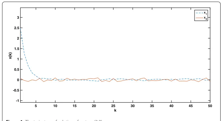
Figure 1The trajectory of solution of system (3.2)

=xT(k)ATAx(k) + 2xT(k)ATGw(k) +wT(k)GTGw(k) –xT(k)ETEx(k)

=

x1(k)

x2(k)

T

0.5 0

0.5 1

0.5 0.5

0 1

x1(k)

x2(k)

+ 2

x1(k)

x2(k)

T

0.5 0

0.5 1

1 1

w(k)

+wT(k)

1 1 1

1

w(k) –

x1(k)

x2(k)

T

1 0

0 0

1 0

0 0

x1(k)

x2(k)

= 0.25x2₁(k) + 0.5x1(k)x2(k) + 1.25x22(k) +x1(k)w(k) + 3x2(k)w(k)

+ 2w(k)2–x1(k)2

= –0.75x2₁(k) + 1.25w2(k) + 0.5x1(k)w(k) –w(k)2

≤–0.75x2₁(k) + 0.25x2₁(k) + 0.25w2(k) + 0.25w(k)2

= –0.75x2₁(k) + 0.25x2₁(k) + 0.25x2₂(k) + 0.25w(k)2

= –0.5x2₁(k) + 0.25x₂2(k) + 0.25w(k)2

= –0.5x2₁(k) – 0.5x2₂(k) + 0.75x2₂(k) + 0.25w(k)2

= –0.5x2₁(k) +x2₂(k)+ 0.75w2₂(k) + 0.25w(k)2

= –0.5x(k)2+w2(k).

Therefore, by Theorem 3.2, we may show that system (3.2) is exponentially practically stable in thepth-moment withη= 35.6,λ= 0.5,r= 0.5. For simulation purpose, we let

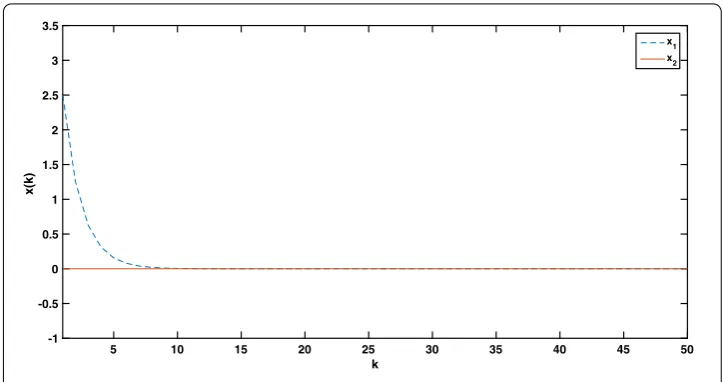
a= 0.3,w(k) ≤0.1. Then Theorem 3.2 is satisﬁed with the parametersc1= 1,c2= 1,a= 0.3,c3= 0.5,p= 2,ρ(w(k)) =w(k)2≤0.01. Figure 1 shows the trajectories of solution of Example 4.1 with disturbance. Figure 2 shows the trajectories of solution of Example 4.1 without disturbance.

Example4.2 Consider system (2.1) withE=1 0_{0 0},A=_{–0.05 –0.05}–0.05 0 ,B=_{–0.05 –0.02}0.4 0 ,G=

_0.5 0.5

(20)

Figure 2The trajectory of solution of system (3.2) without disturbance

A)) =rank(E) = 1. Thus, system (2.1) is regular and causal. For nonsingular matricesM=

_{2 0} 0 2

,N=_{–0.5 –10}0.5 0 , we get

MEN=

1 0

0 0

, MAN=

–0.05 0

0 1

,

MBN=

0.4 0

–0.03 0.4

, MG=

1 1

.

We choose a Lyapunov–Krasovskii functional asV(k,x(k)) =|x1(k)|+awitha> 0.

FromEx(k) =1 0_{0 0}_xx1(k)

2(k)

=x1(k) 0

and

Ex(k+ 1) =

1 0

0 0

x1(k+ 1)

x2(k+ 1)

=

–0.05 0

–0.05 –0.05

x1(k)

x2(k)

+

0.4 0

–0.05 –0.02

x1(k–τ)

x2(k–τ)

+

0.5 0.5

w(k),

we obtain

x1(k+ 1) 0

=

–0.05x1(k) + 0.4x1(k–τ) + 0.5w(k)

–0.05x1(k) – 0.05x2(k) – 0.05x1(k–τ) – 0.02x2(k–τ) + 0.5w(k)

.

Thus, we obtain

(i) Ex(k) ≤V(k,x(k)) =|x1(k)|+a≤ Ex(k)+a,

(ii) IfV(k+s,x(k+s))≤qV(k+ 1,x(k+ 1))withs∈N–τ, then we have

x1(k+ 1) = –0.05x1(k) + 0.4x1(k–τ) + 0.5w(k), _x1(k+ 1)≤0.05x1(k)+ 0.4x1(k–τ)+ 0.5w(k),

(21)

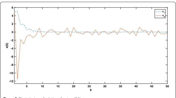
Figure 3The trajectory of solution of system (2.1)

+ 0.5w(k),

x1(k+ 1)+a≤0.05x1(k)+a+ 0.4x1(k–τ)+a+ 0.55a+ 0.5w(k),

Vk+ 1,x(k+ 1)≤0.05Vk,x(k)+ 0.4Vk–τ,x(k–τ)+ 0.55a+ 0.5w(k)

≤0.05Vk,x(k)+ 0.4qVk+ 1,x(k+ 1)+ 0.55a+ 0.5w(k)

≤ 0.05 1 – 0.4qV

k,x(k)+0.55a+ 0.5w(k)

1 – 0.4q .

Thus,

Vk,x(k)=Vk+ 1,x(k+ 1)–Vk,x(k)

≤ 0.05 1 – 0.4qV

k,x(k)+0.55a+ 0.5w(k)

1 – 0.4q –V

k,x(k)

= –

1 – 0.05

1 – 0.4q V

k,x(k)+0.55a+ 0.5w(k) 1 – 0.4q

= –βVk,x(k)+ρw(k),

whereβ≤1 – 0.05

1–0.4qandρ(w(k)) =

0.55a+0.5w(k) 1–0.4q .

Therefore, by Theorem 3.4, system (2.1) is exponentially practically stable in thep

th-moment with η = 82.41,λ= 0.8, and r = 54.58. For simulation purpose, we let a=

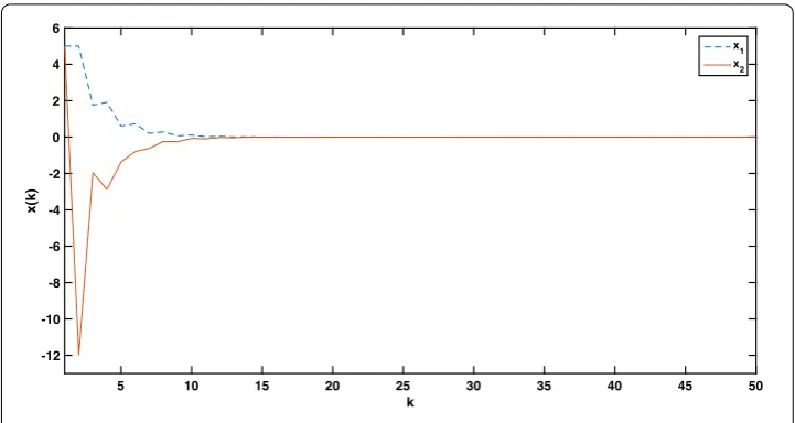
0.5,w(k) ≤0.1. Then Theorem 3.4 is satisﬁed withc1= 1,c2= 1,a= 0.5,q= 1.6,β= 0.8,p= 1,ρ(w(k))≤0.9. Figure 3 shows the trajectories of solution of Example 4.2. Fig-ure 4 shows the trajectories of solution of system (2.1) without disturbance.

5 Conclusion

(22)

respec-Figure 4The trajectory of solution of system (2.1) without disturbance

tively. For systems with delay and disturbances, by using the Razumikhin-type technique, we derived exponentially practical stability criteria for a general discrete time system and a linear singular system, respectively. Numerical examples were given to show eﬀectiveness of our theoretical results.

Acknowledgements

The ﬁrst author is supported by student scholarship from the Human Resources Development in Science Project (Science Achievement Scholarship of Thailand SAST). The second author is supported by Chiang Mai University. This research is also (partially) supported by the Center of Excellence in Mathematics, The Commission on Higher Education, Thailand.

Competing interests

The authors declare that they have no competing interests.

Authors’ contributions

All authors read and approved the ﬁnal manuscript.

Publisher’s Note

Springer Nature remains neutral with regard to jurisdictional claims in published maps and institutional aﬃliations.

Received: 4 September 2017 Accepted: 20 March 2018

References

1. Feng, G., Cao, J.: Stability analysis of impulsive switched singular systems. IET Control Theory Appl.9(6), 863–870 (2015)

2. Feng, Z., Li, W., Lam, J.: New admissibility analysis for discrete singular systems with time-varying delay. Appl. Math. Comput.265, 1058–1066 (2015)

3. Gao, C., Liu, X., Li, W.: Input-to-state stability of discrete-time singular systems based on quasi-min-max model predictive control. IET Control Theory Appl.9(11), 1662–1669 (2015)

4. Han, Y., Kao, Y., Gao, C.: Robust sliding mode control for uncertain discrete singular systems with time-varying delays and external disturbances. Automatica75, 210–216 (2017)

5. Hassanabadi, A.H., Shaﬁee, M., Puig, V.: UIO design for singular delayed LPV systems with application to actuator fault detection and isolation. Int. J. Syst. Sci.47(1), 107–121 (2015)

6. Hien, L.V., Vu, L.H., Phat, V.N.: Improved delay-dependent exponential stability of singular systems with mixed interval time-varying delays. IET Control Theory Appl.9(9), 1364–1372 (2015)

7. Li, S., Lin, H.: Onl1stability of switched positive singular systems with time-varying delay. Int. J. Robust Nonlinear

Control27(16), 1–15 (2017)

8. Li, S., Xiang, Z.: Stabilityl1-gain andl∞-gain analysis for discrete-time positive switched singular delayed systems. Appl. Math. Comput.275, 95–106 (2016)

9. Lin, J., Gao, Z.: Observers design for switched discrete-time singular time-delay systems with unknown inputs. Nonlinear Anal. Hybrid Syst.18, 85–99 (2015)

(23)

11. Liu, Y., et al.: Input-to-state stability for discrete-time nonlinear switched singular systems. Inf. Sci.358(359), 18–28 (2016)

12. Liu, T., et al.: Finite-time stability of discrete switched singular positive systems. Circuits Syst. Signal Process.36(6), 1–13 (2017)

13. Long, S., Zhong, S.: Improved results for stochastic stabilization of a class of discrete-time singular Markovian jump systems with time-varying delay. Nonlinear Anal. Hybrid Syst.23, 11–26 (2017)

14. Ma, Y., Zheng, Y.: Delay-dependent stochastic stability for discrete singular neural networks with Markovian jump and mixed time-delays. Neural Comput. Appl.29(1) 111–122 (2018)

15. Muoi, N.H., Rajchakit, G., Phat, V.N.: LMI approach to ﬁnite-time stability and stabilization of singular linear discrete delay systems. Acta Appl. Math.146(1), 81–93 (2016)

16. Niamsup, P., Phat, V.N.: A new result on ﬁnite-time control of singular linear time-delay systems. Appl. Math. Lett.60, 1–7 (2016)

17. Rami, M.A., Napp, D.: Positivity of discrete singular systems and their stability: an LP-based approach. Automatica 50(1), 84–91 (2014)

18. Sau, N.H., Niamsup, P., Phat, V.N.: Positivity and stability analysis for linear implicit diﬀerence delay equation. Linear Algebra Appl.510, 25–41 (2016)

19. Zamani, I., Shaﬁee, M., Ibeas, A.: Stability analysis of hybrid switched nonlinear singular time-delay systems with stable and unstable subsystems. Int. J. Syst. Sci.45(5), 1128–1144 (2014)

20. Zamani, I., Shaﬁee, M., Ibeas, A.: Switched nonlinear singular systems with time-delay: stability analysis. Int. J. Robust Nonlinear Control25(10), 1497–1513 (2015)

21. Zamani, I., Shaﬁee, M.: Stability analysis of uncertain switched singular time-delay systems with discrete and distributed delays. Optim. Control Appl. Methods36(1), 1–28 (2015)

22. Sun, L., Liu, C., Li, X.: Practical stability of impulsive discrete systems with time delays. Abstr. Appl. Anal.2014, 954121 (2014)

23. Wangrat, S., Niamsup, P.: Exponentially practical stability of impulsive discrete time system with delay. Adv. Diﬀer. Equ. 2016, 277 (2016)

24. Zeng, Z.: Converse Lyapunov theorems for nonautonomous discrete-time systems. J. Math. Sci.161(2), 337–343 (2009)

25. Ghanmi, B., Hadj Taieb, N., Hammami, M.A.: Growth conditions for exponential stability of time-varying perturbed systems. Int. J. Control86(6), 1086–1097 (2013)

26. Ben Hamed, B., Ellouze, I., Hammami, M.A.: Practical uniform stability of nonlinear diﬀerential delay equations. Mediterr. J. Math.8, 603–616 (2011)

27. Ben Hamed, B., Hammami, M.A.: Practical stabilization of a class of uncertain time-varying nonlinear delay systems. J. Control Theory Appl.7(2), 175–180 (2009)

28. Caraballo, T., Hammami, M.A., Mchiri, L.: Practical exponential stability of impulsive stochastic functional diﬀerential equations. Syst. Control Lett.109, 43–48 (2017)

29. Ellouze, I., Hammami, M.A.: Practical stability of impulsive control systems with multiple time delays. Dyn. Contin. Discrete Impuls. Syst., Ser. A Math. Anal.20, 341–356 (2013)

30. Dai, L.: Singular Control Systems. Springer, New York (1989)

31. Chen, W., Lu, X., Zheng, W.: Impulsive stabilization and impulsive synchronization of discrete-time delayed neural networks. IEEE Trans. Neural Netw. Learn. Syst.26(4), 734–748 (2015)