R E S E A R C H
Open Access
Disjoint multi mobile agent itinerary
planning for big data analytics
Bo Liu
1*, Jiuxin Cao
1, Jie Yin
1, Wei Yu
2, Benyuan Liu
3and Xinwen Fu
3Abstract
Sensor networks are often part of a cyber-physical system. A large-scale sensor network often involves big data collection and data fusion. The agent technology has drawn much attention in wireless sensor networks (WSNs) to perform data fusion and energy balancing. Existing multi-agent itinerary algorithms are either time-consuming or too complicated in practice. In this paper, we design a routing itinerary planning scheme for the multi-agent itinerary problem by constructing the spanning tree of WSN nodes. First, we build a multi-agent-based distributed WSN (DWSN) model and energy consumption model. Second, we present a novel routing itinerary algorithm named DMAIP, which can group all the sensor nodes into multiple itineraries for agents. We also extend DMAIP and design DMAIP-E, which can avoid long-distance transmission in DMAIP. Our evaluation results demonstrate that our
algorithms are better in terms of life cycle and energy consumption than the existing DWSN data collecting schemes.
Keywords: Distributed wireless sensor network, Mobile agent, Itinerary planning, Energy efficiency
1 Introduction
Wireless sensor networks have been widely used for data collection [1–3] and situation monitoring in various appli-cations, including environment monitoring, automatic target detection, and tracking in battlefields, forests, farm-lands, and coal mines. To support these applications, we can place sensors at critical locations. The raw data col-lected by sensors can then be forwarded through a num-ber of relay nodes to a remote base station, denoted as sink node [4, 5]. In a WSN, sensor nodes with limited energy are often randomly deployed in massive quantities, and each node may act both as a data collector and a traffic relay, as shown in existing research [4]. Sensor network as a major component of IOT always produces big data [6, 7]. The new techniques make it possible to access more com-putation power and use more energy; but the energy is still limited, and how to “reduce” the big data is still an important problem in WSN.
The agent-based technology has attracted growing attention to improve energy efficiency, scalability, and reliability of a WSN [8–12]. Agent is now playing a use-ful role in IOT because it can execute data fusion tasks
*Correspondence: [email protected]
1School of Computer Science and Engineering, Southeast University, Nanjing, China
Full list of author information is available at the end of the article
autonomously [13], as a result, agent can relieve the net-work load and prolong lifetime [14] of WSNs. In an agent-based WSN, the main technical challenges include data fusion and energy efficiency, as well as energy and load balancing [15]. For example, Lin et al. [16] leveraged the agent-based technology to balance energy consumption in data collection process of WSNs. Mobile agent-based schemes can also reduce the amount of raw data to be transmitted.
A critical agent-based WSN problem is how to design the itinerary through the WSN for mobile agents (MAs) to collect data. Existing approaches for generating agent itineraries can be classified into two categories: (i) sin-gle agent itinerary planning [17–20] and (ii) multi-agent itinerary planning (MIP) [21–23]. For example, Xu et al. [17] investigated static, dynamic, and predictive dynamic schemes to solve the target tracking problem in WSNs. However, the work considers only one target node in the field, their algorithms are based on trilateration, and the itinerary is for only one agent. In reality, using a single agent is not practical because of large delay, unbalanced load, and large accumulated size [21, 22]. Therefore, some researchers try to find solutions for MIP. For example, Chen et al. [21] proposed a source-grouping scheme and an iterative MIP algorithm based on single agent itinerary
planning in order to solve the problem of single agent itinerary planning.
In this paper, we propose a novel multi-agent itinerary planning strategy for WSNs. We also prove that finding optimal balanced disjoint paths for mobile agents to tra-verse the whole WSN is a NP-hard problem. We design a depth-first-search (DFS)-based itinerary algorithm. We construct the spanning tree over the WSN. Our theoret-ical analysis shows that our designed algorithm is simple and easy to realize in comparison with existing multi-itinerary algorithms. We conduct performance evaluation using QualNet [24] and our results indicate that our novel multi-agent itinerary algorithm achieves better perfor-mance than the existing cluster schemes which was always used in cluster-based approaches [12, 25–27]. For exam-ple, better energy balancing and longer life cycle can be obtained in our methods.
The multi-agent itinerary planning (MIP) algorithms proposed in this paper are designed for generic large-scale sensor network. We now give a few scenarios to demon-strate its potential practical use. A typical scenario to apply our algorithms is to monitor an environment that is large and dangerous for human being, such as the environ-ment with possible radiation exposure. For example, radi-ation leak from Tokyo Electric Power’s Fukushima Daiichi nuclear power facility contaminated an area of 12.5 mi. Large-scale sensor networks can also play an important role in monitoring the areas that are endangered by pos-sible debris flows. In those hostile environments, mobile agents can be dispatched from aircrafts.
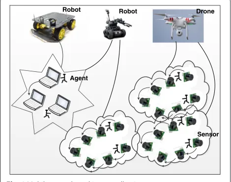
A mobile agent is a physical software which can migrate from one sensor to another or from UAVs (or robots) to sensors. To run the mobile agent, some middleware need to be configured which provide the execution envi-ronment for agents. Mobile agents can also be applied in visual sensor networks, as illustrated in Fig. 1. As
Drone Robot
Robot
Sensor Agent
Fig. 1Mobile agent-based image collection
the technology advances, hardware modules are getting smaller. Such small hardware modules can be integrated into sensor devices for specialized use as add-on compo-nents. Imagery applications are a classical example. For example, the Cyclops image capturing and inference mod-ule can be integrated into popular WSN devices [28]. Mobile agent middleware such as Mobile-C [29] is also available and can be conveniently deployed in sensors, laptops, drones, and other equipments. In Fig. 1, mobile agents carrying image processing codes are dispatched to the target region in order to visit the image sensors according to the arranged itinerary, collecting image data from the corresponding zone of interest. Mobile agents can perform fusion operation over the large volume of imagery data at each sensor node in the target region. Therefore, the mobile agents will be able to migrate, carrying much less load. When the environment of inter-est changes or the sensing task changes, new mobile agents that carry different image processing algorithms can be dispatched to these image sensors to execute new tasks.
The rest of this paper is organized as follows: In Section 2, we present the most related work. In Section 3, we present two models of agent-based WSNs. In Section 4, we propose the energy consumption model. In Section 5, we present the problem. In Section 6, we present the agent routing approach considering energy balancing. In Section 7, we show performance evaluation results. We conclude the paper in Section 8.
2 Related works
proposed scheme is very complicated and not easy to be implemented.
Clustering is an important strategy to solve the data fusion and collection problem in WSNs and has been widely used. For example, in the conventional low-energy adaptive clustering hierarchy (LEACH) [25] algorithm, the high-energy cluster head positions are randomly rotated so that the energy consumption of sensors can be bal-anced. In addition, LEACH assumes a homogeneous dis-tribution of sensor nodes in the given area, which may not be realistic. We will compare our algorithm with clustering-based algorithms [26, 27, 30]. It is worth not-ing that existnot-ing research efforts on multi-agent routnot-ing mainly focus on how to group source nodes to generate itineraries other than how to compute balanced routes. Our work fills this gap.
3 Mobile agent-based wireless sensor networks
In the area of distributed wireless sensor network (DWSN) based on agent, there are commonly two paradigms: (i) single agent-based WSN and (ii) multi-agent-based WSN. In the following, we first present the network models for both WSN with single agent and then WSN with multiple agents.
3.1 Single agent-based WSN
As shown in the Fig. 2, in a single agent-based WSN, the mobile agent will first move from sink node along paths to the cluster head of a target area and will then collect data. After collecting data from one cluster, the mobile agent will move to the next cluster head and collect data. It will not return to sink node until it reaches the last cluster head. In comparison with the traditional centralized data collection manner (all-to-one), it really reduces network energy consumption to a certain degree. Nonetheless, the process tends to take large time and causes big delay in large-scale WSNs.
Ordinary sensor node
Cluster head node
Sink node
Target area
Mobile agent
Fig. 2Single mobile agent data collection model
3.2 Multi-agent-based WSN
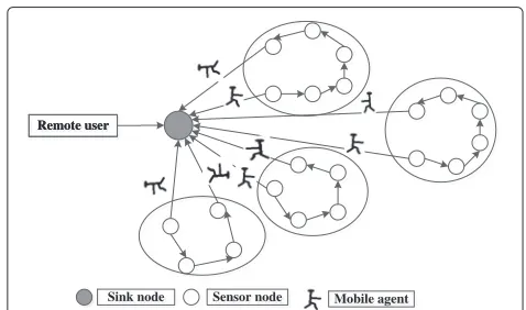
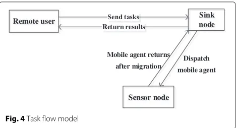
Based on the single agent model, we propose a multi-agent-based data collection scheme. As shown in Fig. 3, there are three components in our scheme:remote user, sink node, sensor node. A remote user assigns tasks to a sink node. All sensor nodes have an operating environ-ment installed for the mobile agent. When the sink node receives a task from a remote user, the sink node traverses network topology to generate a spanning tree, then assigns every path to a mobile agent. When a mobile agent moves along its own path to a sensor node, it will perform the data processing and carry the fused data to the next node. All agents will perform tasks in parallel until they visit all nodes of their paths. The sink node will manipulate data from every path and send back the final results to the remote user. Figure 4 shows the detailed workflow.
4 Energy consumption model
We now present the energy consumption model used in our scheme. In a WSN, sensor nodes will communicate with each other through wireless communication. The design of a network topology control algorithm has a great impact on the energy consumption of a sensor node. To the ordinary sensor node, the longer the data transmis-sion distances among sensor nodes are, the more the loss of radio signal is. Facing long-distance data transmissions, we will adopt the method of multi-hop to transmit data in order to save energy.
We adopt the energy consumption model in [31–33] as the single sensor node energy model. The energy con-sumption for sending data (ETx) consists of the energy consumed by an amplifier circuit (ETx-amp) and by a trans-mission circuit (ETx-elec), while the energy consumption for receiving data is composed of the energy consumed by a receiving circuit (ERx-elec). Based on this, we consider the energy computation for the cluster-based WSN model and the multi-agent-based WSN model in the following.
We consider two modes for energy consumption when sending data: free space transmission mode and multi-hop
Remote user
Sink node Sensor node Mobile agent Remote user
Remote user nodeSink
Fig. 4Task flow model
attenuation mode. The mode that we choose depends on the distancedbetween the sending node and the receiving node. Ifdis larger than thresholdd0, the multi-hop atten-uation mode will be chosen. If dis smaller than d0, the free space transmission mode will be used. Also, denotel as the size of data packet.
The computational formula of the energy consumption of sending node(ETx)is
The computational formula of the energy consumption of receiving node(ERx)is
ERx(l)=ERx-elec(l)=l∗Eelec (2) In this model, the value of parameterEelecis the energy consumed by transmitting one bit data; it depends on the methods of channel coding and signal propagation. The typical values of parameters accepted by researchers are
Eelec=50 nJ/bit (3)
εamp=0.0013 pJ/bit/m4 (4)
εfs=10 pJ/bit/m2 (5)
According to [18], given a communication node energy consumption model, the energy consumption consists of three parts: energy for controlling data exchange ECtr, energy for receiving dataERx, energy for sending dataETx. Because every node has the same energy consumption for controlling data exchange, we will ignore it in comparison. Therefore, the total energy consumption(Esum)of every node is
wherelr is the size of received data packet, andlt is the
size of transmitted data packet.
Accordingly, we will use the energy formula introduced above to compute the energy consumption of two models: a cluster-based WSN model, a multi-agent-based WSN model.
4.1 Energy consumption of cluster-based WSN
In this kind of algorithm such as LEACH algorithm, wire-less sensor networks have sink node, cluster head node, and ordinary member node. Here, we assume that clus-ter head node has ability of fusing data and the rate of fusion is p. Ordinary member node sends raw data to its cluster head. Cluster head receives data from every cluster member from two parts: (1) ordinary cluster mem-ber nodes and (2) cluster head nodes. Assume that every cluster member node has a data packet whose size is l, and that cluster member nodes send data to the cluster head node, and that only sending data consumes energy. From the energy model formula above, we have the energy consumption of cluster member:
Assume every cluster head hasNcluster members. The energy consumption of cluster head is divided into two parts: one is for receiving data from cluster members and the other is for sending gathered data to the sink node. So the energy consumption for receiving data (EcluRev) will be
as follows.
EcluRev=N∗l∗Eelec (8)
Energy consumption for sending data (EcluTran) is:
EcluTran=
[(N∗(1−p)+1)]∗l∗(Eelec+εfsd2), d<d0
[(N∗(1−p)+1)]∗l∗(Eelec+εampd4), d≥d0
(9)
We can know that the total energy consumption of cluster head is
Eclu=EcluTran+EcluRev (10)
4.2 Energy consumption of multi-agent-based WSN
There are only sink node and ordinary sensor nodes in wireless sensor networks. During the process of data col-lection, a mobile agent will collect and fuse the data of each node. Assume that the size of a mobile agent islMA, and the size of data packet collected from every sensor node isl. Here, we also assume that cluster head node has ability of fusing data and the rate of fusion isp. When the mobile agent reaches thekth node, the size of the data in total is
So the energy consumption of thekth node for sending
The energy consumption for receiving data is
Er=lk−1∗Eelec (13)
So the total energy consumption of thekth node is
E=Et+Er (14)
5 Problem definition
Mobile agents can improve data fusion, energy man-agement, and topology management and have attracted great attention in the WSN research. Generally speak-ing, mobile agents can use raw data on remote sensor nodes, balance the energy consumption of sensor nodes, and improve the reliability by extending the network life cycle.
Given a WSN, we utilize mobile agent techniques to accomplish data collection and fusion with less energy consumption and longer life cycle. A sink node (e.g., base station) is responsible for gathering data from sensor nodes in the WSN. The objective of our research is to find multiple disjoint paths (MDP) with balanced length which cover all sensor nodes in the WSN. The disjoint paths will be assigned to mobile agents.
Definition 1(MDP problem). Given an undirected con-nected graphG =< V, E, W >, whereV is the set of nodes andEis the set of edges, the number of nodes inV isn,W = {w1, w2, ..., wm}is a set of weights
correspond-ing to every edge inE. The problem is to findk disjoint paths inGto cover allnnodes inV, where every edge in these paths can be found inE, and to make the longest path (the one with the maximum sum of weights among all the paths) minimized.
In the following, we will prove the MDP problem is NP-hard. To prepare for the proof, we firstly give the formal definition of the partition problem which is known as a NP-hard problem.
Definition 2(Partition problem). Givennpositive inte-gersa1,a2, ,an. The problem is to make the integers be
partitioned into two subsetsAandBsuch that the sum of the integers inAequals the sum of the integers inB, that
is
ai∈A
ai= aj∈B
aj(1≤i,j≤n).
Theorem 1. MDP problem is NP-hard.
Proof.We prove this theorem by constructing a polynomial-time reduction from the partition problem to MDP problem.
Firstly, we create a positive integerMandMis satisfied
with the following equation:M>
n
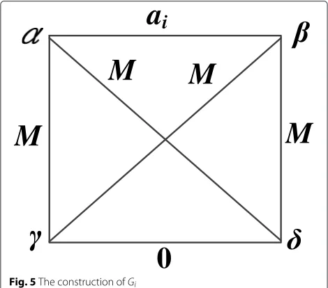
Secondly, For everyai, we construct a small undirected
weighed graphGiwith four vertexes as shown in Fig. 5.
Note that, if this small graph is divided into two parts, thenα andβ must be in the same part; otherwise, there will be one edge with weight M in the one part of the graph.
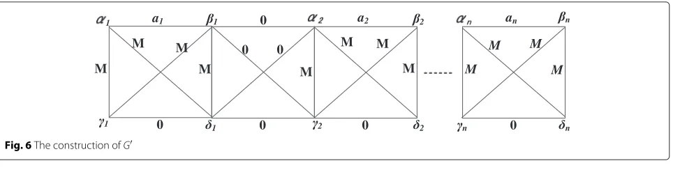
Thirdly, the small graphs are connected and constructed into a big graphG, as shown in Fig. 6.
From Fig. 6, we can see that the connection between the small graph of a1and the small graph of a2is specially designed as zero weight edges. Obviously,α2andγ2must be in two parts, soβ1will be together withα2in the same part or be together withγ2in the same part. The rest can be done in the same manner. As a result, G is divided into two parts, and every part has a path including 2n ver-texes whose length is the sum of some integers. The total number of vertexes inGis 4n.
The partition problem has the solution if and only if the graphGcan be divided into two parts and every part has 2nvertexes; the length of the path passing these vertexes is
not more thann
i=1(
ai)2. Here, the 4nis corresponding to
thenin the MDP problem; the 2nis corresponding to the kof the MDP problem. So, we have successfully reduced the partition problem to the example of MDP problem in polynomial time. Theorem 1 holds.
M
M
M
M
Fig. 6The construction ofG
Since it is NP-hard to find optimal number of disjoint paths with balanced length, we focus on developing effi-cient heuristic and polynomial time algorithms to make agents work effectively in a WSN and produce near-optimal itineraries.
6 Algorithms for multi-agent itinerary
We now present a novel DFS-based multi-agent itinerary planning (DMAIP) algorithm in WSNs. Particularly, we first present the DMAIP algorithm that reduces the com-munication distance between sensor nodes in the agents’ migration path. Then, we present the enhanced DMAIP algorithm, denoted as DMAIP-E. DMAIP-E changes the process of traversing the network, considering the dis-tance between the sink node and sensors when disjoint paths are generated to balance the length of paths.
6.1 DMAIP algorithm
In DMAIP algorithm, we first build a network topology graph based on WSN. We then generate a spanning tree of the connected graph in the order of increasing weight and finally traverse the spanning tree recursively to find disjoint paths of all the subtrees.
Algorithm 1 introduces how we build the network topologyG. We assume that the wireless sensor nodes can locate themselves. They will send position coordinates to the sink node. Accordingly, the sink node will collect posi-tion data and compute distances between all the pairs of nodes. If the distance is not larger than the radius, we leave it as what it is. Otherwise, we will mark it inaccessible explicitly by value−1.
Algorithm 2 generates a spanning tree of the connected graph G. Basically, we traverse the connected graph or weighted adjacent matrixMby DFS and generate a span-ning tree including all nodes in the graph.
In Algorithm 3, we traverse the spanning tree recur-sively to find disjoint paths of all the subtrees.
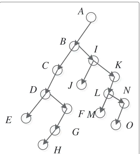
There is an example in Fig. 7 to illustrate the generation of paths more clearly. We begin preorder traversal from nodeA, where we get the first pathA−B−C−D−E. Then, we go back to nodeF, getting the second pathF−G−H. Then, the third path isI−J. The forth path isK−M. The last path isN−O. As a result, we obtain 5 disjoint paths:
Algorithm 1Build a network topology graphG. Input: Arrayc[n] [ 2] andR
//cincludes n nodes’ two-dimension coordinates.Ris the communication radius.
Output:Weighted adjacent matrixM=[du,v]n∗n
//du,vis the distance between nodeuandv.
Algorithm description: Calculate distance between all pairs of the nodes. Assumeuandvare two nodes, then their distance is:
du,v=
(c[u] [ 0]−c[v] [ 0])2+(c[u] [ 1]−c[v] [ 1])2 (15)
Ifdu,v ≤ Ror u = sink or v = sink, then leave du,v
as what it is, elsedu,v = −1. Ifu = v,du,v = −1. It
is obvious thatdu,v = dv,u. At last, we get matrixM =
[du,v]n∗n.
(1)A−B−C−D−E, (2)F−G−H, (3)I−J, (4)K−M, (5)N−O.
At last, we get disjoint paths including all the sensor nodes in network topology graph. We can send each path to an agent to travel along.
6.2 DMAIP-E algorithm
If the sensor node is far away from the sink node, energy consumption increases and this will reduce the lifetime of the WSN. In DMAIP, it is possible to generate such paths that are very long and the end nodes of which may be far away from the sink node. In order to avoid these long paths, we consider the distance between the sink node and sensor nodes during DFS. Based on DMAIP, we propose an algorithm called DMAIP-E that considers the distance between the sink node and all sensor nodes, as shown in Algorithm 4. We first build the network topology graph according to Algorithm 1 of DMAIP to obtain the distance matrixM = (du,v)n∗n. We then generate multiple paths
for agents.
Algorithm 2Generate a spanning tree of the connected graphG.
Input: Weighted adjacent matrixM=[du,v]n∗n
Output: A connected spanning treeT Algorithm description:
Define an array storing visited states of nodes as S[i](1≤i≤n). Initialize all values to zero except that S[sink]=1.
(1) Chooseu0 from all sensor nodes wheredu0,sink is
minimum, as the initial start node or source node. (2) Visit nodeu0,preu=u0,u=u0.
Track back to the last nodepreuto
find the nextvofpreu; GOTO (5).
IF there is no such nodevTHEN GOTO (7). (5) Create an undirected edge fromutov,
preu=u,S[preu]=1 andu=v.
(6) GOTO (4). (7) End.
//The order of visited nodes form a spanning tree. A spanning tree is generated after all nodes visited.
Algorithm 3Generate disjoint paths from TreeT. Input: A connected spanning treeT
Output:Several disjoint pathsP1· · ·Pk.
Algorithm description:
//We will achieve this algorithm by calling the function GeneratePath.
GeneratePath(TreeNode & rootNode) Begin
TreeNode subtreeRootNodes[];
Find the path along from rootNode to the left-most node;
Store the path as one disjoint path;
Delete the left-most child and all nodes in the path; Store all nodes in the path that still have child node(s) in subtreeRootNodes[];
Forevery subtreeRootNodes[i] GeneratePath(subtreeRootNodes[i]); End for;
End
path during this process. We begin with the nearest node A to the sink node; find the next node B that meets Formula 16.
Fig. 7An example for generation of disjoint path
We illustrate the process of choosing appropriate node Bin Fig. 8. NodeBmust be satisfied with Formula 16. So nodes 1, 2, and 3 are being considered. Besides, we require the nearest node to nodeA. Therefore, node 2 is the node B. Assume nodeBas the nextAand find the next node B. Once there is no more nodeBto be found, it will form a path from the first nodeAto the last nodeB. Then, go
Algorithm 4 Generate multiple disjoint paths when traversing.
Input: Weighted adjacent matrixM=(du,v)n∗n
Output:A group of disjoint pathsP1· · ·Pk.
Algorithm description:
Define an array storing visited states of nodes as S[i](1≤i≤n).
InitializeS[i] with 0 except thatS[sink]=1.
step (1)WithinM, find the nearest nodeA0to the sink node.
A=A0
step (2) S[A]= 1, and then find the appropriate node B.
step (3) A = B, S[A]= 1, and then find the next appropriate nodeB.
step (4)Repeat step (3) until we cannot find the next B. Store the path from the firstAto the lastBas a new path.
Sink
A
1
2
3
Fig. 8A process of choosing appropriate node B
back to the sink node and repeat the process above. It will stop when all nodes are included in all generated paths.
The sink node will dispatch an agent to the farthest node of every disjoint path generated above. When an agent fin-ished its task, it will return from the other end of its path to the sink node, and the sink node will manipulate all data from all paths before sending it back to the remote user. In fact, we let the sink node dispatch agents to the outer-most location of the path to decrease the distance that the agent loaded with data migrates.
The time complexity of DMAIP algorithm isO(n3). The time complexity of DMAIP-E algorithm isO(n2).
7 Performance evaluation
We implemented the DMAIP and DMAIP-E schemes in the Qualnet environment [20] and compared them with LEACH algorithm which is the basic of some existing algorithms [26, 27, 30]. We evaluated the performance of the proposed algorithms using the energy model stated in Section 4. Finally, we presented the experimental results of comparing DMAIP, DMAIP-E, and LEACH.
7.1 Simulation setup
We deployed sensor nodes randomly in an area of 200 m×200 m. Each node was deployed at a fixed posi-tion. Sink node is located at (100,100). Table 1 gives the parameter settings.
We take the following assumptions: (i) a WSN is of large scale and nodes are distributed randomly, (ii) the initial energy batteries of all the sensor nodes are the same, (iii) the data packet is of the same size, and (iv) all sensor nodes stay in the fixed position.
In this paper, we focused on the data collection pro-cess of sensor nodes in WSNs and proposed mobile agent-based schemes to improve the performance of data collection process. We evaluate the performance of our proposed schemes in terms of energy efficiency and life
Table 1Simulation experimental parameter settings
Parameter name Value
Number of nodes 50, 75, 100, 125, 150
Size of the area/m2 200×200
Location of the base station/m (100, 100)
Initial energyEinit/J 0.5
Energy consumption of transmitting amplifier 10 Efs/(pJ∗bit−1∗m−2)
Energy consumption of transmitting amplifier
0.0013 Eamp/(pJ∗bit−1∗m−4)
Energy consumption of transmitting and receiving 50 circuitEelec/nJ∗bit−1
Initial size of mobile agent /byte 1024
Length of data packet/byte 2048
Data fusion ratep 0.9
Communication radius/m 40
cycle. In the following, we first compare three related algorithms and then show their performance results.
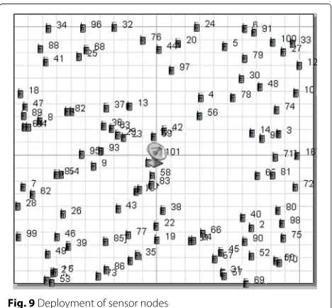
The clustering mechanism and multi-path mechanism are different representative algorithms for data collection in a WSN. All LEACH-based algorithms use a cluster-ing mechanism for data collection, while our proposed DMAIP and DMAIP-E use multi-path mechanism. The WSN consists of 100 sensor nodes. In our experiments, the three algorithms run in the same environment. Ini-tially, all sensor nodes are deployed as shown in Fig. 9.
Itineraries of LEACH algorithm: In LEACH algorithm, we choose 13 sensor nodes as cluster heads from 100 ones. Ordinary nodes can only communicate with cluster heads,
and only cluster heads can communicate with sink nodes. Figure 10 illustrates the results for LEACH-based algo-rithms. According to the LEACH strategy, ordinary nodes will choose the nearest cluster head as theirs because of the randomness of deployed sensor nodes and cluster head nodes. Therefore, each cluster head node manages unbalanced number of ordinary nodes within its domain. For example, there are 2 cluster members in the 86th cluster, while there are 11 cluster members in the 49th cluster. A cluster head may communicates with many clus-ter members and may have long communication distance with the sink node. This phenomenon leads to a fast death of some cluster heads due to the fast energy consump-tion. With the increasing number of the sensor nodes in large-scale WSNs, the distance between a cluster head, its cluster member nodes, and sink node will be larger and consume much more energy. Therefore, LEACH is appropriate for relatively small WSNs.
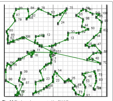
Itineraries of DMAIP and DMAIP-E algorithms: Figure 11 illustrates the results for DMAIP. It has 4 paths and the last node along each path consumes the most energy. For example, in Fig. 11, the 70th node, the last node of a path, is far from the sink node and dies fast because of the fast energy consumption. Figure 12 shows the results for DMAIP-E algorithm. Recall that DMAIP-E algorithm is the enhanced version of the DMAIP algo-rithm and considers not only the distance between nodes but also the distance between the last node of each path and sink node. The sink node dispatches mobile agents to the farthest end of each path, and the agent returns to the other end of the path. This reduces the amount of energy consumption to a certain degree and extends the life cycle of the wireless sensor network.
Fig. 10The branches generated by LEACH
Fig. 11The branches generated by DMAIP
7.2 Simulation metrics and results
To evaluate the performance from our simulation results, the following three performance metrics are considered: life cycle, energy consumption, and impact of the number of nodes. Table 2 gives the evaluation metrics.
Life cycle: From Fig. 13, we can see that with the different number of nodes, the life cycle of DMAIP-E is much longer than that of DMAIP, and the lifetime of DMAIP is a little longer than that of LEACH algo-rithm as the communication distance of DMAIP-E is the smallest, while the distance of LEACH is mostly very large.
Table 2Performance metrics
Evaluation metrics Descriptions
Round The whole process from when the sink node dispatch agents for every path for data collection to when all agents return to the sink node with their data.
Energy consumption of network nodes
The total energy consumption by sensor nodes when sink node completes one round of data collection.
Number of remaining nodes
The number of sensor nodes alive in the network.
Life cycle The round number from the beginning of the network to the death of the first node.
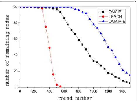
The number of residual nodes: Figure 14 illustrates results, which present the number of remaining nodes ver-sus the number of rounds. As we can see from Fig. 14, as the number of rounds increases, some sensor nodes will die. The number of rounds for LEACH, DMAIP, and DMAIP-E to have dead nodes are 250, 280, and 650, respectively. DMAIP-E has the largest number of rounds, i.e., the longest life cycle, more than twice the rounds of the other two algorithms. The reason why nodes in DMAIP die very early is that it is very far from the end node of some paths to the sink node and therefore trans-mitting data from the end node to the sink node will consume energy heavily. In addition, all nodes for LEACH die in about 600th round, while for DMAIP and DMAIP-E, nodes will not be all dead until about 1500th round. This is because DMAIP and DMAIP-E adopt a mobile agent model, which could save and balance the energy of sensor nodes. Also, DMAIP-E outperforms other schemes.
Energy consumption: Energy consumption is another important performance metric for WSNs. This experi-ment was performed in a network with 100 nodes, and
Fig. 13Life cycle with different number of nodes
Fig. 14Changes of residual nodes’ number with rounds increasing
the results are shown in Fig. 15. As we can see from the figure, for every round, the energy consumption of DMAIP and DMAIP-E algorithm is almost the same while the energy consumption of LEACH is not sta-ble. This is because DMAIP and DMAIP-E collect data according to preset paths while LEACH chooses clus-ter heads randomly and changes it every few rounds. Therefore, energy consumption of LEACH is different in different round. The energy consumption of LEACH is not stable because clusters are randomly formed with-out periodic mode. In every round, DMAIP-E algorithm consumes the least energy while LEACH uses the most.
8 Conclusions
The itinerary planning problem is a key issue in dis-tributed WSNs. In this paper, we presented a multi-agent-based paradigm for data collecting in WSN. Because the optimal multi-agent itinerary generation problem is
NP-hard, we proposed an approximate algorithm called DMAIP-E based on the global topology graph. Our sim-ulation results show that DMAIP-E is appropriate for large-scale WSN and has better performance than exist-ing clusterexist-ing-based algorithms in terms of both life cycle and energy consumption.
Competing interests
The authors declare that they have no competing interests.
Acknowledgements
This work is supported by the National Natural Science Foundation of China under Grant Nos. 61370208, 61472081, 61320106007, and 61272531, China National High Technology Research and Development Program (2013AA013503), NSF under award CNS-1527303, SGCC Science and Technology Program “key technologies and application of test platform for dispatching automation system”, Collaborative Innovation Center of Social Safety Science and Technology, Collaborative Innovation Center of Wireless Communications Technology, Jiangsu Provincial Key Laboratory of Network and Information Security (BM2003201), and Key Laboratory of Computer Network and Information Integration of Ministry of Education of China under Grant No. 93K-9.
Author details
1School of Computer Science and Engineering, Southeast University, Nanjing, China.2Department of Computer and Information Sciences, Towson University, Baltimore, USA.3Department of Computer Science, University of Massachusetts Lowell, Lowell, USA.
Received: 24 November 2015 Accepted: 4 April 2016
References
1. S Ji, Z Cai, Distributed data collection in large-scale asynchronous wireless sensor networks under the generalized physical interference model. IEEE Trans. Netw.21(4), 1270–1283 (2013)
2. S Chen, M Huang, S Tang, Y Wang, Distributed data collection in large-scale asynchronous wireless sensor networks under the generalized physical interference model. IEEE Trans. Parallel Distributed Syst.21(4), 52–60 (2012)
3. S Ji, R Beyah, Z Cai, Snapshot and continuous data collection in probabilistic wireless sensor network. IEEE Trans. Mobile Comput.13(3), 626–637 (2014)
4. F Wang, D Wang, JC Liu, inProceedings of the 6th Annual IEEE Communications Society Conference on Sensor, Mesh and Ad-HoC
Communications and Networks. Traffic-aware relay node deployment for
data collection in wireless sensor networks, (Rome, Italy, 2009), pp. 351–359
5. H Luo, Y Liu, SK Das, Distributed algorithm for en route aggregation decision in wireless sensor networks. IEEE Trans. Mobile Comput.8(1), 1–13 (2009)
6. A Zaslavsky, C Perera, D Georgakopoulos, inProceedings of the
International Conference on Advances in Cloud Computing, ACC 2012.
Sensing as a service and big data, (Bangalore, India, 2012), pp. 21–29. http://citeseerx.ist.psu.edu/viewdoc/summary?doi=10.1.1.294.9753 7. T-M Choi, HK Chan, X Yue, Recent development in big data analytics for
business operations and risk management. IEEE Trans. Cybernet.
2016(99), 1–12 (2016)
8. H Qi, X Wang, SS Iyengar, K Chakrabarty, inProceedings of the 5th
International Conference on Information Fusion. Multisensor data fusion in
distributed sensor networks using mobile agents, (Singapore, 2001), pp. 11–16. http://citeseerx.ist.psu.edu/viewdoc/summary?doi=10.1.1.10. 7251
9. W Du, J Deng, YS Han, PK Varshney, inProceedings of the 10th ACM
conference on Computer and communications security (CCS 2003). A
pairwise key pre-distribution scheme for wireless sensor networks, (Washington, DC, USA, 2003), pp. 42–51. http://dl.acm.org/citation.cfm? id=948118
10. L Eschenauer, VD Gligor, inProceeding of the 9th ACM Conference on
Computer and Communications Securit (CCS ’02). A key-management
scheme for distributed sensor networks, (Washington, DC, USA, 2002), pp. 41–47. http://dl.acm.org/citation.cfm?id=586117
11. H Qi, Y Xu, X Wang, Mobile-agent-based collaborative signal and information processing in sensor networks. Proc. IEEE.91(8), 1172–1183 (2003)
12. E Amiri, H Keshavarz, AS Fahleyani, H Moradzadeh, S Komaki, inIEEE International Conference on Space Science and Communication (IconSpace
2013). New algorithm for leader election in distributed WSN with software
agents, (Melaka, Malaysia, 2013), pp. 290–295. http://ieeexplore.ieee.org/ xpls/abs_all.jsp?arnumber=6599483
13. L Jarvenpaa, M Lintinen, A-L Mattila, in17th International Conference on
System Theory, Control and Computing (ICSTCC). Mobile agents for the
internet of things, (Sinaia, Romania, 2013), pp. 763–767. http://ieeexplore. ieee.org/xpls/abs_all.jsp?arnumber=6689053
14. J Chen, S He, Y Sun, et al., Optimal flow control for utility-lifetime tradeoff in wireless sensor networks. Comput. Netw.53(18), 3031–3041 (2009) 15. C Wu, GS Tewolde, W Sheng, B Xu, Y Wang, Distributed multi-actuator
control for workload balancing in wireless sensor and actuator networks. IEEE Trans. Automatic Control.56(10), 2462–2467 (2011)
16. K Lin, M Chen, S Zeadally, JJPC Rodrigues, Balancing energy consumption with mobile agents in wireless sensor networks. Future generation computer systems. Future Generation Comput. Syst.28(2), 446–456 (2012)
17. Y Xu, H Qi, Mobile agent migration modeling and design for target tracking in wireless sensor networks. Ad Hoc Netw.6(1), 1–16 (2008) 18. M Chen, L Yang, T Kwon, L Zhou, Itinerary planning for energy-efficient
agent communications in wireless sensor networks. IEEE Trans. Vehic. Technol.60(7), 3290–3299 (2011)
19. B Chen, W Liu, Mobile agent computing paradigm for building a flexible structural health monitoring sensor network. Computer-aided Civil Infrastruct. Eng.25(7), 504–516 (2010)
20. Q Wu, NSV Rao, J Barhen,et al, On computing mobile agent routes for data fusion in distributed sensor networks. IEEE Trans. Knowl. Data Eng.
16(6), 740–753 (2004)
21. M Chen, S Gonzalez, Y Zhang, VCM Leung, Multi-agent itinerary planning for wireless sensor networks. Lecture Notes Inst. Comput. Sci. Soc. Informatics Telecommun. Eng.22, 584–597 (2009)
22. W Cai, M Chen, T Hara, L Shu, inProceeding of the 5th Annual International
Wireless Internet Conference (WICON). Ga-mip: Genetic algorithm based
multiple mobile agents itinerary planning in wireless sensor network, (Singapore, 2010)
23. A Mpitziopoulos, D Gavalas, C Konstantopoulos, G Pantziou, CBID: a scalable method for distributed data aggregation in WSNs. Int. J. Distributed Sensor Netw.2010(206517), 13 (2010)
24. N SQ, Scalable Network Technologies. Inc. Available: www.qualnet.com. (2011)
25. WR Heinzelman, A Chandrakasan, H Balakrishnan, inIEEE Proceedings of the 33rd Annual Hawaii International Conference on System
Sciences(HICSS-33). Energy-efficient communication protocol for wireless
microsensor networks, (Maui, Hawaii, USA, 2000), pp. 1–10. http:// ieeexplore.ieee.org/xpl/articleDetails.jsp?arnumber=926982 26. R Malhotra, R Aggarwal, S Monga, Analyzing core migration protocol
wireless ad hoc networks. Int. J. Comput. Appl.9(3), 35–41 (2010) 27. CE Nugraheni, Formal verification of ring-based leader election protocol
using predicate diagrams. Int. J. Comput. Sci. Netw. Secur.9(8), 1–8 (2009) 28. IF Akyildiz, T Melodia, K Chowdhury, A survey on wireless multimedia
sensor networks. Int. J. Comput. Telecommun. Netw.4, 921–960 (2007) 29. B Chen, HH Cheng, J Palen, Mobile-C: a mobile agent platform for mobile
C(C++) agents. Software-Prac. Exp.15, 1711–1733 (2006)
30. A Galstyan, B Krishnamachari, K Lerman, inWorkshop on Sensor Networks
at the 19th National Conference on Artificial Intelligence (AAAI-04). Resource
allocation and emergent coordination in wireless sensor networks, (San Jose, California, USA, 2004), pp. 114–118. http://www.isi.edu/~galstyan/ papers/wsn-RA.pdf
31. YK Xiao, XM Shan, Y Ren, Game theory models for IEEE802.11 dcf in wireless ad hoc networks. IEEE Communications Magazine.43(3), S22–S26 (2005)
32. C-C Tseng, K-C Chen, Y-J Liang, Z-W Tuanand, inThe 65th IEEE Vehicular
cluster- based network architectures for wireless ad hoc networks, (Dublin, Ireland, 2007), pp. 114–118. http://ieeexplore.ieee.org/stamp/ stamp.jsp?tp=&arnumber=4212464
33. ZL C, RJ M, W A, inIEEE International Conference on Communications. An integrated data-link energy model for wireless sensor networks, (Paris, France, 2004), pp. 3777–3783. http://ieeexplore.ieee.org/stamp/stamp. jsp?tp=&arnumber=1313260
Submit your manuscript to a
journal and benefi t from:
7Convenient online submission 7Rigorous peer review
7Immediate publication on acceptance 7Open access: articles freely available online 7High visibility within the fi eld
7Retaining the copyright to your article