R E S E A R C H
Open Access
Discrete Fourier transform based frequency
characteristics of iterative learning control for
linear discrete-time systems
Xiaohui Li
1and Xiaoe Ruan
1**Correspondence:
[email protected] 1School of Mathematics and
Statistics, Xi’an Jiaotong University, Xi’an, P.R. China
Abstract
For discrete-time iterative learning control systems, the discrete Fourier transform (DFT) is a powerful technique for frequency analysis, and Toeplitz matrices are a typical tool for the system input–output transmission. This paper first exploits z-transform and DFT-based frequency properties for iterative learning control systems and studies the convergence property of a Toeplitz matrix to the power of iteration index. The exploitation exhibits that for the finite-length discrete-time iterative learning control systems, the time-domain convolution theorem for thez-transform and DFT is no longer true, and the Toeplitz matrix to the power of iteration index converges if and only if the identical diagonal element lies in the unit circle. Then, by considering the DFT to a finite-length sequence as a linear transform, it is easy to equivalently reform the input–output equation of linear discrete time-invariant and time-varying ILC systems as an algebraic discrete-frequency equation. Thus the derivative-type (D-type) iterative learning control (ILC) converges in a
discrete-frequency domain if and only if it converges in a discrete-time domain. Numerical simulations are carried out to exhibit the validity and effectiveness.
Keywords: Iterative learning control; Discrete Fourier transform; Monotone convergence; Linear discrete systems; Power formula
1 Introduction
Since the iterative learning control (ILC) has been invented three decades before, it has been acknowledged as an efficacious intelligent strategy for a robot manipulator to repet-itively execute a desired trajectory tracking over a finite time interval [1–3]. The mech-anism is iterative generating an upgrading control input for the next iteration by means of compensating the control input at the current iteration with its proportional, integral, and/or derivative tracking discrepancy between the current output and the desired tra-jectory [4–12]. The pursuing aim is that the generated control input may drive the system to track the desired trajectory as precise as possible as the iteration index goes on, or in other words, the ILC is convergent.
Reviewing the contributions of the ILC convergence for discrete-time systems, the an-alytical techniques are mainly the time- and frequency-domains. In terms of convergence in a discrete-time domain, the kernel idea is to express the ILC dynamics as an algebraic input–output equation by the lift vector technique, and thus the ILC convergence is
alent to the stability of the transmit matrix as shown [13–26]. The idea is innovative, and the results are progressive. However, the convergence only involves the asymptoti-cal tracking behavior measured in the sense of some fixed norm [26,27] but does not much concerns with the transient performance evolution along the iteration axis. In fact, it is worth noticing that the input–output transmit matrix of a linear ILC-driven system is Toeplitz, and thus along the iteration axis the evolution behavior of the Toeplitz ma-trix to the power of iteration index must convey the learning performance evolution be-haviors, including the transient overshooting, asymptotical convergence, or convergence monotonicity. Therefore the inherent significant property of the Toeplitz matrix is advan-tageous to ILC convergence analysis in a direct manner but not well discussed yet. This paper addresses it.
Despite the ILC convergence explorations in the time domain, the ILC convergence analysis in the frequency domain is necessary for filtering and cut-off frequency computa-tion. For this, one existing analytical technique is thez-transform as adopted in [28–31], where thez-transform-based frequency-domain ILC convergence and robustness have been made basing on the postulation that the time-domain convolution theorem holds, which converts the convolution of two infinite-length discrete-time sequences into an al-gebraic multiplication of twoz-transforms. However, as the input and output of a discrete-time ILC-driven system are of finite length, thez-transform, which is fit to an infinite-length signal [32], may not precisely deliver the frequency information. In the authors’ opinion, iis regarded as an approximate computation. This opinion has also been com-mented in [33].
a given input, the precision of an unstable system is worse than that of a stable system because the energy loss of the last part information of an unstable system is larger.
Actually, by virtue of the repetition feature of the ILC system, the iteration-wise out-put can be regarded as a segment of a periodic sequence whereas for a periodic sequence, the DFT is a well-known powerful technique, which expresses the sequence with the fun-damentalN period as a summation of a fundamental sine wave plus (N– 1) harmonic sine waves. Its equivalent form is in exponential complex-variable functions. Then the frequency-domain spectrum can be precisely computed by DFT in a direct manner. This motivates the paper firstly to investigate DFT properties for linear discrete time-invariant (LDTI) derivative-type (D-type) ILC systems and the convergence of the Toeplitz matrix to the power of the iteration index. The followed works are the frequency-domain con-vergence derivation of LDTI D-type ILC systems and its generalization to linear discrete time-varying (LDTV) D-type ILC systems.
The rest of the paper is organized as follows. Section 2exhibits properties of thez -transform and DFT for truncated LDTI systems together with convergence property of Toeplitz matrix to the power of iteration index. Section 3 presents frequency-domain convergence analysis of LDTI and LDTV D-type ILC systems, respectively. Numerical simulations are made in Sect.4, and Sect.5concludes the paper.
2 z-Transform and DFT for truncated LDTI systems 2.1 z-Transform feature of truncated LDTI systems
Definition 1 (z-transform and inverse z-transform [32]) For a sequence {h(n)}n=+∞ n=0 =
{h(0),h(1), . . . ,h(n), . . .}, itsz-transform is defined as
ˆ
h(z) =Zh(n)=
+∞
n=0
h(n)z–n, Rh–<|z|<Rh+,
where z is a complex variable, and Rh–<|z|<Rh+ refers to the region of convergence (ROC).
Then the inversez-transform ofhˆ(z) is defined as a contour integration:
h(n) =Z–1hˆ(z)= 1 2πj
c
ˆ
h(z)zn–1dz,
whereCrepresents a closed contour within the ROC:Rh–<|z|<Rh+andj2= –1.
By derivation it is easy to testify the additivity and homogeneity for bothz-transform and inversez-transform.
Lemma 1 (Time-domain convolution theorem [32]) Given {w(n)}n=0n=+∞ def= {h(n) ∗
v(n)}n=+n=0∞={w(n) =nl=0h(n–l)v(l)}n=0n=+∞,we havewˆ(z) =hˆ(z)ˆv(z) =vˆ(z)hˆ(z),provided that the z-transform-based frequency domain input–output dynamics for a discrete linear time-invariant system takes the form
ˆ
y(z) =gˆ(z)uˆ(z), (1)
By the time-domain convolution theorem the discrete time-domain dynamics of system (1) is equivalently formulated as
y(n+ 1) =
n
l=0
g(n+ 1 –l)u(l) forn∈N={0, 1, 2, . . .}, (2)
wherey(n) =Z–1(ˆy(z)),g(n) =Z–1(ˆg(z)), andu(n) =Z–1(uˆ(z)).
Let I = [ε1|ε2| · · · |εN] denote theNth-order unit matrix, and let S = [ε2|ε3| · · · |εN|0] be
a shift matrix.
Proposition 1 Sl= [εl+1|εl+2| · · · |εN|0| · · · |0]for l= 2, 3, . . . ,N– 1andSN=0.
Define the truncation operator
(Φ[n1,n2]x)(n) =
⎧ ⎨ ⎩
x(n), n1≤n≤n2,
0, otherwise.
Here the integer (n2–n1+ 1) is the assigned truncation length. Denote the lifted vectors as
Φ[1,N]y=
(Φ[1,N]y)(1)|(Φ[1,N]y)(2)| · · · |(Φ[1,N]y)(N) T
,
Φ[0,N–1]u=
(Φ[0,N–1]u)(0)|(Φ[0,N–1]u)(1)| · · · |(Φ[0,N–1]u)(N– 1) T
.
Then
Φ[1,N]y=
y(1)|y(2)| · · · |y(N)T,
Φ[0,N–1]u=
u(0)|u(1)| · · · |u(N– 1)T.
Define the matrix operator for a truncation as
M(Φ[1,N]w)def= W =w(1)I +w(2)S +· · ·+w(N)SN–1,
whereΦ[1,N]w= [w(1)|w(2)| · · · |w(N)]T.
Proposition 2 εl= Sl–1ε1for l= 2, 3, . . . ,N,andSW= WS.Hereεl= Sl–1ε1is assigned as the(l– 1)th shift impulse signal.
By making the truncation operator to system (2), a lift-vector form description becomes
Φ[1,N]y= M(Φ[1,N]g)Φ[0,N–1]u.
Denote the z-transform truncations with respect to the sequences {(Φ[1,N]y)(n)},
{(Φ[0,N–1]u)(n)}, and{(Φ[1,N]g)(n)}as
(Φ[1,N]gˆ)(z) =g(1) +g(2)z–1+· · ·+g(N)z–(N–1),
(Φ[0,N–1]uˆ)(z) =u(0) +u(1)z–1+· · ·+u(N– 1)z–(N–1).
Proposition 3 The relationship of the z-transform truncations with respect to(2)is as
follows:
(Φ[1,N]ˆy)(z) – (Φ[1,N]gˆ)(z)(Φ[0,N–1]uˆ)(z)
= –g(N)u(1) +g(N– 1)u(2) +· · ·+g(2)u(N– 1)z–N
–g(N)u(2) +g(N– 1)u(3) +· · ·+g(3)u(N– 1)z–(N+1)
–· · ·–g(N)u(N– 1)z–2(N–1).
Proof
(Φ[1,N]ˆy)(z) =y(1) +y(2)z–1+· · ·+y(N)z–(N–1)
=g(1)u(0) +g(2)u(0) +g(1)u(1)z–1
+· · ·+g(N)u(0) +g(N– 1)u(1) +· · ·+g(1)u(N– 1)z–(N–1). (3)
Additionally,
(Φ[1,N]gˆ)(z)(Φ[0,N–1]uˆ)(z)
=g(1) +g(2)z–1+· · ·+g(N)z–(N–1)u(0) +u(1)z–1+· · ·+u(N– 1)z–(N–1)
=g(1)u(0) +g(2)u(0) +g(1)u(1)z–1
+· · ·+g(N)u(0) +g(N– 1)u(1) +· · ·+g(1)u(N– 1)z–(N–1)
+g(N)u(1) +g(N– 1)u(2) +· · ·+g(2)u(N– 1)z–N
+g(N)u(2) +g(N– 1)u(3) +· · ·+g(3)u(N– 1)z–(N+1)
+· · ·+g(N)u(N– 1)z–2(N–1). (4)
Taking Eqs. (3) and (4) into account achieves the result.
2.2 Discrete Fourier transform for LDTI SISO systems
Definition 2(Discrete Fourier transform [32]) For a finite-length discrete sequencev=
[v(0)|v(1)| · · · |v(N– 1)]T, its discrete Fourier transform (DFT) is defined as
Its inverse discrete Fourier transform (IDFT) takes the form
v(n) = 1
Analogously, its inverse discrete Fourier transform (IDFT) (6) can be rewritten as
v(n) = 1
It is no difficult to derive the famous Parseval energy formula
Moreover,
V(N–m)=V(–m)=V(m). (8)
We further calculate the DFT for a class of LDTI single-input–single-output (SISO) sys-tems described by
whereN is a finite positive integer denoting the total sampling number,x(n),u(n), and
y(n) arep-dimensional state vector, scalar input, and scalar output, respectively, and A, B, and C are matrices of appropriate dimensions.
Letu∗=ε1= [1 0 · · · 0]T be the impulse signal and stimulate systems (9). Then the
output takes the form
y∗=g1=g1(1)|g1(2)| · · · |g1(N)T=CB|CAB|CA2B| · · · |CAN–1BT,
where the vectorg1is assigned as the impulse response of system (9).
Thus, for any inputu= [u(0)|u(1)| · · · |u(N– 1)]T, the output of system (9) is expressed
Then
Comparing the summation expression on the right side of Eq. (11) with that of (12), we ob-serve that usualyY+(m)=G
1(m)U(m) unlessN= +∞. This means that the time-domain
convolution theorem for the discrete Fourier transform applied to a finite-length sequence is not true either. The expressionG1(m)U(m) is only regarded as an approximation of
Y+(m). Therefore, the so-called approximate spectrum-based convergence and robust-ness in [34–41] need to be refined in a rigorous manner.
For an example, in the LDTI SISO system (9), denote the spectral radius of thepth-order state matrix A asρ(A) =max1≤i≤p{|λi|}withλi,i= 1, 2, . . . ,p, being the eigenvalues of A.
For simplicity, denote byY˜(m) =G1(m)U(m) the frequency-domain output approxima-tion of the precise frequency-domain outputY+(m).
LetY+2=
the 2-norms of the frequency-domain output, frequency-domain approximate output, and time-domain output, respectively. From Parseval’s energy formula (7) we haveY+
2=
√
Ny+2.
For comparison, generate an input sequence u= [u(0)|u(1)| · · · |u(79)]T with
compo-nents being uniformly distributed random numbers between 0 and 1.
Case 1: Let hibits the frequency-wise magnitude spectra of the frequency-domain output and its ap-proximation when the truncation lengthN= 20, from which we see that| ˜Y(m)|<|Y+(m)|
for frequency orders m= 1, 2, . . . , 19 but| ˜Y(0)|>|Y+(0)|. Figure2 displays the energy
Figure 2Energy tendency of output and its approximation
Figure 3Magnitude spectrum of output and its approximation
tendencies of the frequency-domain output, frequency-domain approximate output, and time-domain output as the truncation lengthNincreases, which says that the discrepancy of the approximation ˜Y2from the precise valueY+2enlarges as the truncation length Nincreases.
Case 2: Let
A=
⎡ ⎢ ⎣
0.8869 0 0
0.1507 0.7989 1 0.0008 0.100 0.7
⎤ ⎥
⎦, B=
⎡ ⎢ ⎣
0 0.0097 0.0093
⎤ ⎥
⎦, C=0 0 1
.
It is testified thatρ(A) = 0.8869 < 1. This implies that the system is stable.
Figure3depicts the frequency-wise magnitude spectra of the output and its approxima-tion when the truncaapproxima-tion lengthN= 20, which conveys that the orders of frequency-wise spectra|Y+(m)|and| ˜Y(m)|are diverse. Whilst Fig.4presents the 2-norms of
frequency-domain output, frequency-frequency-domain approximate output, and time-frequency-domain output for the truncation lengthsN= 10, 20, . . . , 80, respectively, which shows that the discrepancy of the approximation ˜Y2from the precise valueY+2does not distinctly enlarge as the
truncation lengthNincreases.
Besides, Figs.1and3deliver that|Y+(m)|=|Y+(N–m)|and| ˜Y(m)|=| ˜Y(N–m)|for
m= 1, 2, . . . , 19, whereas Figs.2and4convey thatY+ 2≡
√
Ny+ 2.
2.3 Relationship formulation in discrete-frequency domain
Figure 4Energy tendency of output and its approximation
For simplicity, denote
y=y+=y(1)|y(2)| · · · |y(N)T,
u=u(0)|u(1)| · · · |u(N– 1)T,
¯ G=
⎡ ⎢ ⎢ ⎢ ⎢ ⎢ ⎢ ⎢ ⎣
g1(1) 0 0 · · · 0
g1(2) g1(1) 0 · · · 0
g1(3) g1(2) g1(1) · · · 0
..
. ... ... . .. ...
g1(N) g1(N– 1) g1(N– 2) · · · g1(1) ⎤ ⎥ ⎥ ⎥ ⎥ ⎥ ⎥ ⎥ ⎦
.
From (10) we have
y=G¯u
=G¯u(0)ε1+u(1)ε2+· · ·+u(N– 1)εN
=u(0)G¯ε1+u(1)G¯ε2+· · ·+u(N– 1)G¯εN. (13)
Denote
gl=G¯εl forl= 1, 2, . . . ,N
and
¯
G= [G¯1| ¯G2| · · · | ¯GN].
ThenG¯l=gl=G¯εlforl= 2, . . . ,N, which means that thelth column of the matrixG¯ is the
response of system (10) with respect to the shift impulseεl, named as the (l– 1)th shift
impulse response. HenceG¯ is called the impulse response matrix. Then (10) becomes
y=G¯u= [g1|g2| · · · |gN]u.
Therefore
= [Qg1|Qg2| · · · |QgN]Q–1Qu
= [G1|G2| · · · |GN]Q–1U, (14)
whereGl= [Gl(0)|Gl(1)| · · · |Gl(N– 1)]T= Qglforl= 1, 2, . . . ,N, which expresses the DFT
of the (l– 1)th shift impulse response, and
Gl(m) = N–1
n=0
gl(n+ 1)s–m·n form= 0, 1, 2, . . . ,N– 1. (15)
Denote G = [G1|G2| · · · |GN]. Equivalently, Eq. (14) becomes
Y= GQ–1U. (16)
Equation (16) formulates the discrete-frequency relationship of output, shift impulse re-sponses, and input.
2.4 Properties of Toeplitz matrix
Proposition 4 For a lower triangular Toeplitz matrix
M=
⎡ ⎢ ⎢ ⎢ ⎢ ⎢ ⎢ ⎢ ⎣
a1 0 0 · · · 0
a2 a1 0 · · · 0
a3 a2 a1 · · · 0
..
. ... ... . .. ...
aN aN–1 aN–2 · · · a1 ⎤ ⎥ ⎥ ⎥ ⎥ ⎥ ⎥ ⎥ ⎦
,
we havelimk→+∞Mk=0iffλ=|a1|< 1.
Proof In view of the expression
M=a1I+a2S+a3S2+· · ·+aNSN–1, (17)
denote P =a2+a3S+a4S2+· · ·+aNSN–2. Then PS = SP and Mk= (a1I+ PS)k.
Then, for an indexk(k<N), Eq. (17) induces
Mk= (a1I+ PS)k
= (a1)kI+C1k(a1)k–1PS+· · ·+Ckl(a1)k–lPlSl
+· · ·+Ckk–1(a1)Pk–1Sk–1+ PkSk. (18)
For a sufficiently large iteration indexk(k≥N), by considering SN =0Eq. (18) results in
Mk= (a1I+ PS)k
= (a1)kI+C1k(a1)k–1PS+· · ·+Cki(a1)k–lPlSl
+· · ·+CkN–1(a1)k–(N–1)PN–1SN–1, (19)
whereCkl=k(k–1)l(l–1)······(k–l+1)2·1 .
Sufficiency: Recall the assumption thatλ=|a1|< 1.
By multiple adopting L. Hospital’s rule for limiting times, we have
lim
Remark2 It should be pointed out that Proposition4can be regarded as a corollary of Schur complementary. However, the derivation of Schur complementary is too compli-cated to easily acquire the evolution of elements of the Toeplitz matrix to the power of iteration index as the power indexk increases. The proof of Proposition4is given in a straightforward mode, which explicitly presents the evolution of elements of the Toeplitz matrix to the power of iteration index in a clear way. This is helpful in observing the evolu-tion behavior of the transient learning performance of the iterative learning control system because the transmit matrix of the tracking errors of the two adjacent iterations turns to be a lower triangular Toeplitz matrix.
Proposition 5 If the matricesM1andM2are Toeplitz,thenM1M2= M2M1is Toeplitz.
Proposition 6 For a lower triangular matrix
Proof Leta1=maxi=1,2,...,N{|ai,i|}andal+1=maxi=1,2,...,N–l{|ai+l,i|}forl= 1, 2, . . . ,N– 1.
Then
–M≤–|R| ≤R≤ |R| ≤M,
where|A|= (|aij|)≤ |B|= (|bij|) if and only if|aij| ≤ |bij|.
By multiplication of matrices it is no difficult to yield
–Mk≤Rk≤Mk.
From Proposition4we havelimk→+∞Rk=0.
3 Convergence analysis
3.1 DFT-based convergence for LDTI systems 3.1.1 First-order D-type ILC scheme and convergence
Provided that system (10) attempts to track a predetermined desired trajectoryyd(n+ 1) while it repetitively operates, letu1(n) be an arbitrary initial input, and lete1(n+ 1) =yd(n+ 1) –y1(n+ 1) denote the output error of systems (10) driven byu1(n),n= 0, 1, 2, . . . ,N– 1. By compensatingu1(n) with its output errore1(n+ 1),u2(n) is generated. In recursion, the first-order derivative-type iterative learning control (D-type ILC) updating law is for-mulated as
u1(n), arbitrary given,
uk+1(n) =uk(n) +Γek(n+ 1), n= 0, 1, 2, . . . ,N– 1,
(20)
where the subscriptk= 1, 2, . . . denotes the iteration index, andΓ is assigned as the deriva-tive learning gain.
Denote
yd=yd(1)|yd(2)| · · · |yd(N)T,
uk=
uk(0)|uk(1)| · · · |uk(N– 1)T,
yk=yk(1)|yk(2)| · · · |yk(N) T
,
ek=yd–yk=ek(1)|ek(2)| · · · |ek(N) T
,
Yk= Qyk,
Ek= Qek,
Uk= Quk.
Inferring the derivation of Eq. (14), we have
yk=G¯uk. (21)
Analogously, the first-order D-type ILC (20) becomes
Theorem 1 Assume that for system(10)g1(1)= 0,and the first-order D-type ILC(22)is applied.Then in the frequency domain,limk→+∞Ek+1=0if and only ifρ1=|1 –Γg1(1)|< 1.
Proof Taking Eqs. (21) and (22) into account yields
ek+1= (I –ΓG)¯ ek. (23)
Then
Ek+1= Qek+1= Q(I –ΓG)Q¯ –1Qek= Q(I –ΓG)Q¯ –1Ek. (24)
Therefore
Ek+1= Q(I –ΓG)Q¯ –1Ek= Q(I –ΓG)¯ 2Q–1Ek–1=· · ·= Q(I –ΓG)¯ kQ–1E
1. (25)
In Eqs. (23) and (24),
I–ΓG¯ =
⎡ ⎢ ⎢ ⎢ ⎢ ⎢ ⎢ ⎢ ⎣
1 –Γg1(1) 0 0 · · · 0
–Γg1(2) 1 –Γg1(1) 0 · · · 0
–Γg1(3) –Γg1(2) 1 –Γg1(1) · · · 0 ..
. ... ... . .. ...
–Γg1(N) –Γg1(N– 1) –Γg1(N– 2) · · · 1 –Γg1(1)
⎤ ⎥ ⎥ ⎥ ⎥ ⎥ ⎥ ⎥ ⎦
. (26)
Noting that the matrix I –ΓG¯ is lower triangular Toeplitz, from Proposition4the
suffi-ciency and necessity are immediate.
Remark3 Because the matrix Q is invertible,limk→+∞Ek+1=0in the discrete-frequency
domain if and only iflimk→+∞ek+1=0in the discrete-time domain. This is theoretically logic and thus convincing. Thus the robustness of the ILC algorithm to the system param-eters uncertainty may be addressed in the time domain in a direct manner. This issue is involved in our future work. As for the existing frequency-domain convergence analysis by means of thez-transform, the convergence equivalence to the discrete-domain result is quite obscure, the robustness analysis such as of the system parameter uncertainty by thez-transform needs to be refined in a rigorous manner, as mentioned in Remark1.
Remark4 Though the frequency-domain relationship of (16) is not simpler than the rela-tionship in the time domain, Theorem1of the paper conveys that the lifted tracking error vector converges itself. This means that the tracking error may converge while measured in any form of norm. This is benefited from the property of the lower triangular Toeplitz matrix addressed by Proposition4. However, in many existing convergence results, the discrete-time convergence of the traditional D-type iterative learning control algorithm is ensured in the sense of the lifted tracking error measured in some of but not a preferred norm.
Remark5 The derivation of Theorem1conveys that the convergence conditionρ1=|1 –
learning gainΓ, but no relevance to the system matrix A. This coincides with the existing conclusion in the literature [31].
Remark6 From the proof of Lemma1 we found that the magnitude of tracking error would grow extremely at the first finite iterations. This makes the use of ILC cautious for practical applications. A preferred candidate guarantees the ILC algorithm (22) to be monotonously convergent.
Theorem 2 Assume that the D-type ILC(22)is applied to system(10)and satisfies the conditionρ˜1=I–ΓG¯2< 1.ThenEk+12<Ek2andlimk→+∞Ek+12= 0.
Proof Calculating the 2-norm of both sides of expression (23), we have
ek+12≤ I–ΓG¯2ek2. (27a)
From Parseval’s energy formula (7), (27a) is equivalently reformed as
Ek+12≤ I–ΓG¯2Ek2. (27b)
According to the 2-norm of matrix I –ΓG,¯
I–ΓG¯2=
ρ(I –ΓG)¯ T(I –ΓG)¯ ,
whereρ((I –ΓG)¯ T(I –ΓG)) =¯ max
i(λi((I –ΓG)¯ T(I –ΓG))) denotes the spectral radius of¯
the matrix (I –ΓG)¯ T(I –ΓG).¯
Considering the assumptionρ˜1=I–ΓG¯2< 1, the results are ensured.
Remark7 From the above-mentioned convergence condition, the choice of learning gain
Γ is one degree of freedom but depends upon the impulse response at all sampling in-stants. This makes the choice of learning gainΓ difficult. For the regard, a possible manner is to adaptively construct a time-varying iteration-dependent ILC algorithm.
3.2 DFT-based convergence for LDTV systems
Consider the class of LDTV systems described as
⎧ ⎪ ⎪ ⎨ ⎪ ⎪ ⎩
x(n+ 1) = A(n)x(n) + B(n)u(n),
y(n+ 1) = C(n+ 1)x(n+ 1),
x(0) =0, n= 0, 1, . . . ,N– 1;
(28)
whereNis the total sampling number,x(n),u(n), andy(n) arep-dimensional state vector, scalar input, and output, respectively, and A(n), B(n), and C(n) are time-varying matrices of appropriate dimensions.
Letu∗=ε1= [1 0 · · · 0]Tbe the impulse signal and stimulate systems (28). Then the
output takes the form
whereg1˜ (1) = C(1)B(0) andg1˜ (l) = C(l)(l–1i=1A(i))B(0) forl= 2, 3, . . . ,N. The vectorg1˜ is assigned as the impulse response of LDTV system (28).
Thus, for any inputu= [u(0)|u(1)| · · · |u(N– 1)]T, its output is expressed as
Next, we derive a discrete-frequency relationship among output, shift impulse re-sponses, and input for LDTV system (28).
Denote
impulse response. Then (29) becomes
y=Hu= [g˜1|˜g2| · · · |˜gN]u.
Therefore
= [Qg˜1|Qg˜2| · · · |Qg˜N]Q–1Qu
= [G1|G2| · · · |GN]Q–1U, (31)
whereGl= [Gl(0)|Gl(1)| · · · |Gl(N– 1)]T= Qg˜lforl= 1, 2, . . . ,N, which expresses the DFT
of the (l– 1)th shift impulse response, and
Equation (33) formulates the discrete-frequency relationship of output, shift impulse re-sponses, and input.
Comparing the input–output equation (33) for LDTV system (28) with the input–output equation (16) for LDTI system (10), the constructive forms of the input–output transmit matrices are identical, except that the elementsGl(m) expressed by (32) are different from
Gl(m) given by (15). By considering the difference and using Proposition6, we analogously achieve the following convergence results.
Theorem 3 Assume that,for system(28),gl˜(1)= 0,l= 1, 2, . . . ,N,and the first-order D-type ILC(22)is applied.Then,in the frequency domain,limk→+∞Ek+1=0if and only if
ρ2=maxl=1,2,...,N|1 –Γg˜l(1)|< 1.
Remark8 Theorem3reveals that the convergence is guaranteed in the vector form either for the time-domain tracking error or for the frequency-domain tracking error. This im-plies that the tracking error converges in any form of norm. However, the existing results are only for a fixed but unknown norm [26,27], although they are equivalent.
Theorem 4 Assume that the D-type ILC(22)is applied to system(28)and satisfies the conditionρ˜2=I–ΓH2< 1.ThenEk+12<Ek2andlimk→+∞Ek+12= 0.
Remark9 Theorem4obtains frequency-domain sufficient conditions for the monotonic convergence of a class of LDTV D-type ILC systems, whilst the z-transform-based fre-quency analysis is very hard to compute the tracking error spectrum either for the infinite-length or for the finite-infinite-length time-varying system. The result is marvelous for practical applications.
4 Numerical simulations
Example1 Consider the LDTI SISO system
Figure 5Tracking behavior of the D-type ILC
Figure 6Tracking error tendency in discrete-time domain
The sampling number of system (34) is set asD¯ ={0, 1, 2, . . . , 99}. The desired trajectory is chosen asyd(n) = 1 –exp(–0.048n),n∈ ¯D, and the beginning control input is chosen as
u1(n) = 1,n∈ ¯D. The initial state is set asxk(0) = [xk1(0),x2k(0),x3k(0)]T= [0, 0, 0]T. It is
ob-vious thatek(0) = 0. For the D-type ILC algorithm (22), we choose the derivative learning
gainΓ = 40. It is computed thatρ1=|1 –Γg1(1)|= 0.9276, which means that the
conver-gent conditionρ1< 1 holds.
Figure5exhibits the tracking behavior of system (34) driven by the D-type ILC (22), where the dash curve stands for the desired trajectory, and the dash-dotted and solid ones are the outputs at the fiftieth and eightieth iterations, respectively, which shows that the output tracks the desired trajectory closer as the iteration goes on. Figure 6
depicts the tracking error tendency along iteration direction in the sense of 2-norm of ek2=
100
n=1|ek(n)|2in the discrete-time domain.
Figure7exhibits the frequency-wise spectra of the tracking error at the fiftieth, eight-ieth, and hundredth iterations, respectively. Figure 8displays the tracking error energy
tendency expressed byEk2=99m=0|Ek(m)|2.
Example2 Consider the other LDTI SISO system
⎧ ⎪ ⎪ ⎪ ⎨ ⎪ ⎪ ⎪ ⎩
x1k(n+1) x2k(n+1)
=–0.04 0.941 0.02 x 1
k(n)
x2k(n)
+0.020 uk(n),
yk(n) =[0 1]
x1k(n) x2k(n)
, n∈ ¯D.
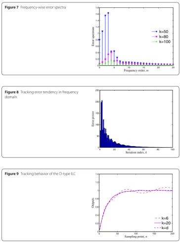
Figure 7Frequency-wise error spectra
Figure 8Tracking error tendency in frequency domain
Figure 9Tracking behavior of the D-type ILC
The sampling time of system (35) is set as D¯ ={0, 1, 2, . . . , 199}. The desired trajectory is given asyd(n) = 1 –exp(–0.048n),n∈ ¯D, and the beginning control input is fixed as
u1(n) = 1,n∈ ¯D. The initial state is set asxk(0) = [x1k(0),x2k(0)]T= [0, 0]T. It is obvious that ek(0) = 0. For the D-type ILC algorithm (22), we select the derivative learning gainΓ = 5.6.
It is computed thatρ˜1=I–ΓG¯2= 0.9423, which means that the monotone convergence
conditionρ˜1< 1 holds.
Fig-Figure 10 Tracking error tendency in discrete-time domain
Figure 11 Frequency-wise error spectra
Figure 12 Tracking error tendency in frequency domain
ure10depicts the monotone convergence of the tracking errorek2= 200
n=1|ek(n)|2
produced by the D-type ILC (22) in the discrete-time domain.
Figure11exhibits the frequency-wise spectra of the tracking error at the sixth, twenti-eth, and thirtieth iterations, respectively, which shows that, for each harmonic frequency
2π
200m, the spectrum|Ek(m)|is decreasing as the iteration indexkincreases. Figure12
dis-plays the monotone convergence of the tracking error powerEk2=199m=0|Ek(m)|2in
the discrete-frequency domain.
5 Conclusion
iterative learning control systems, the time-domain convolution theorem either for thez -transform or for the DFT form is no longer true by rigorous reduction. This challenges the existing methodologies and results in deed. Though the derived DFT-based frequency-domain relationship among the input, impulse response, and the output looks compli-cated, it objectively reveals their inherent features, and thus it is not difficult to achieve the equivalence of the convergence in the frequency domain to the existing results in the time domain. Besides, the adopted DFT-based frequency technique is feasible for linear discrete time-variable systems. This will greatly extend the applicable scope. In addition, the convergences for LDTI systems and for LDTV systems have been made in a straight-forward manner by means of investigating the convergence property of a Toeplitz matrix to the power of iteration index. This is important for an ILC system to present its tracking behavior evolution along the iteration direction. However, this paper does not involve the frequency-domain robustness to system uncertainties and external noise perturbations. This will be addressed in future works.
Acknowledgements
The authors sincerely thank the referees for their suggestions and comments.
Funding
This work was supported by the National Natural Science Foundation of China (No. F010114-61273135).
Competing interests
The authors declare that they have no competing interests.
Authors’ contributions
Both authors contributed equally and significantly in writing this paper. Both authors read and approved the final manuscript.
Publisher’s Note
Springer Nature remains neutral with regard to jurisdictional claims in published maps and institutional affiliations.
Received: 22 September 2018 Accepted: 29 January 2019
References
1. Uchiyama, M.: Formulation of high-speed motion pattern of a mechanical arm by trial. Trans. Soc. Instrum. Control Eng.14(6), 706–712 (1978)
2. Arimoto, S., Kawamura, S., Miyazaki, F.: Bettering operation of robots by learning. J. Robot. Syst.1(2), 123–140 (1984) 3. Arimoto, S., Kawamura, S., Miyazaki, F., Tamaki, S.: Learning control theory for dynamical systems. In: Proc. 24th IEEE
Conf. Decis. Control, vol. 24, pp. 1375–1380 (1985)
4. Bristow, D.A., Tharayil, M., Alleyne, A.G.: A survey of iterative learning control. IEEE Control Syst. Mag.26(3), 96–114 (2006)
5. Moore, K.L., Chen, Y., Ahn, H.S.: Iterative learning control: a tutorial and big picture view. In: Proc. 45th IEEE Conf. Decis. Control, vol. 45, pp. 2352–2357 (2006)
6. Ahn, H.S., Chen, Y.Q., Moore, K.L.: Iterative learning control: brief survey and categorization. IEEE Trans. Syst. Man Cybern., Part C, Appl. Rev.37(6), 1099–1121 (2007)
7. Wang, Y., Gao, F., Doyle, F.J.: Survey on iterative learning control, repetitive control, and run-to-run control. J. Process Control19(10), 1589–1600 (2009)
8. Xu, J.X.: A survey on iterative learning control for nonlinear systems. Int. J. Control84(7), 1275–1294 (2011) 9. Ruan, X.E., Park, K.H., Bien, Z.Z.: Retrospective review of some iterative learning control techniques with a comment
on prospective long-term learning. Control Theory Appl.29(8), 966–973 (2012)
10. Shen, D., Wang, Y.: Survey on stochastic iterative learning control. J. Process Control24(12), 64–77 (2014) 11. Nageshrao, S.P., Lopes, G.A.D., Jeltsema, D., Babuška, R.: Port–Hamiltonian systems in adaptive and learning control:
a survey. IEEE Trans. Autom. Control61(5), 1223–1238 (2015)
12. Shen, D.: Iterative learning control with incomplete information: a survey. IEEE/CAA J. Autom. Sin.5(5), 885–901 (2018)
13. Bu, X., Hou, Z., Hou, Z., Yang, J.: Robust iterative learning control design for linear systems with time-varying delays and packet dropouts. Adv. Differ. Equ.2017(1), 84 (2017)
14. Norrlöf, M., Gunnarsson, S.: Time and frequency domain convergence properties in iterative learning control. Int. J. Control75(14), 1114–1126 (2002)
16. Jeong, G.M., Choi, C.H.: Iterative learning control for linear discrete time nonminimum phase systems. Automatica
38(2), 287–291 (2002)
17. Moore, K.L., Chen, Y.Q., Bahl, V.: Monotonically convergent iterative learning control for linear discrete-time systems. Automatica41(9), 1529–1537 (2005)
18. Tian, S., Liu, Q., Dai, X., Zhang, J.: A PD-type iterative learning control algorithm for singular discrete systems. Adv. Differ. Equ.2016(1), 321 (2016)
19. Li, X.D., Ho, J.K.L., Chow, T.W.S.: Iterative learning control for linear time-variant discrete systems based on 2-D system theory. IEE Proc., Control Theory Appl.152(1), 13–18 (2005)
20. Liu, Y., Jia, Y.: Robust formation control of discrete-time multi-agent systems by iterative learning approach. Int. J. Syst. Sci.46(4), 625–633 (2015)
21. Zhu, Q., Hu, G.D., Liu, W.Q.: Iterative learning control design method for linear discrete-time uncertain systems with iteratively periodic factors. IET Control Theory Appl.9(15), 2305–2311 (2015)
22. Ding, J., Cichy, B., Galkowski, K., Rogers, E., Yang, H.Z.: Robust fault-tolerant iterative learning control for discrete systems via linear repetitive processes theory. Int. J. Autom. Comput.12(3), 254–265 (2015)
23. Xu, Y., Shen, D., Bu, X.: Zero-error convergence of iterative learning control using quantized error information. IMA J. Math. Control Inf.34(3), 1061–1077 (2016)
24. Liu, J., Ruan, X.: Networked iterative learning control for discrete-time systems with stochastic packet dropouts in input and output channels. Adv. Differ. Equ.2017(1), 53 (2017)
25. Liang, C., Wang, J., Shen, D.: Iterative learning control for linear discrete delay systems via discrete matrix delayed exponential function approach. J. Differ. Equ. Appl.24(11), 1756–1776 (2018)
26. Yang, S., Xu, J.X., Huang, D., Tan, Y.: Optimal iterative learning control design for multi-agent systems consensus tracking. Syst. Control Lett.69(2), 80–89 (2014)
27. Bu, X., Hou, Z., Cui, L., Yang, J.: Stability analysis of quantized iterative learning control systems using lifting representation. Int. J. Adapt. Control Signal Process.31(9), 1327–1336 (2017)
28. Gunnarsson, S., Norrlöf, M.: On the design of ILC algorithms using optimization. Automatica37(12), 2011–2016 (2001) 29. Owens, D.H., Hatonen, J.J., Daley, S.: Robust monotone gradient-based discrete-time iterative learning control. Int.
J. Robust Nonlinear Control19(6), 634–661 (2009)
30. Paszke, W., Rogers, E., Gałkowski, K.: Experimentally verified generalized KYP lemma based iterative learning control design. Control Eng. Pract.53, 57–67 (2016)
31. Hatonen, J.J., Moore, K.L., Owens, D.H.: An algebraic approach to iterative learning control. Int. J. Control77(1), 45–54 (2004)
32. Oppenheim, A.V., Schafer, R.W.: Discrete-Time Signal Processing, 3rd edn. Prentice Hall, Englewood Cliffs (2009) 33. Wang, D., Ye, Y., Zhang, B.: Practical Iterative Learning Control with Frequency Domain Design and Sampled Data
Implementation. Springer, Singapore (2014)
34. Freeman, C.T., Lewin, P.L., Rogers, E., Owens, D.H., Hatonen, J.J.: Discrete Fourier transform based iterative learning control design for linear plants with experimental verification. J. Dyn. Syst. Meas. Control131(3), 031006 (2009) 35. Alsubaie, M.A., Freeman, C.T., Cai, Z., Lewin, P., Rogers, E.: ILC initial input selection with experimental verification. In:
Proc. IEEE Symposium on Learning Control at IEEE CDC, pp. 1–6 (2009)
36. Freeman, C.T., Alsubaie, M.A., Cai, Z., Rogers, E., Lewin, P.L.: Model and experience-based initial input construction for iterative learning control. Int. J. Adapt. Control Signal Process.25(5), 430–447 (2011)
37. Meng, D., Jia, Y., Du, J., Yu, F.: Robust learning controller design for MIMO stochastic discrete-time systems: an
H∞-based approach. Int. J. Adapt. Control Signal Process.25(7), 653–670 (2011)
38. Owens, D.H., Hatonen, J.J., Daley, S.: Robust monotone gradient-based discrete-time iterative learning control. Int. J. Robust Nonlinear Control19(6), 634–661 (2010)
39. Paszke, W., Rogers, E., Galkowski, K.: Robust finite frequency design of iterative learning control schemes. IFAC-PapersOnLine49(13), 169–174 (2016)
40. Ge, X., Stein, J.L., Ersal, T.: A frequency-dependent filter design approach for norm-optimal iterative learning control and its fundamental trade-off between robustness, convergence speed and steady state error. J. Dyn. Syst. Meas. Control140(2), 021004 (2018).https://doi.org/10.1115/1.4037271