Title: An Effective Approach for Error Reducing Framework for Localizing Jammers in Wireless Networks

Available Online atwww.ijcsmc.com

International Journal of Computer Science and Mobile Computing

A Monthly Journal of Computer Science and Information Technology

ISSN 2320–088X

IJCSMC, Vol. 4, Issue. 6, June 2015, pg.481 – 488

RESEARCH ARTICLE

An Effective Approach for Error Reducing

Framework for Localizing Jammers in

Wireless Networks

Bhavana S.G., Chandrakala

Assistant Profeccesor CSE Dept.VTU PG Centre, Kalaburagi, India

CSE Dept.VTU PG Centre, Kalaburagi, India

[email protected], [email protected]

Abstract— In wireless sensor networks (WSNs), jamming attacks have become a great concern recently. Finding the location of a jamming device is important so as to take security actions against the jammer and restore the network communication. In this paper, we take a comprehensive study on the jammer localization problem, and designed a framework which localizes one or multiple jammers with high accuracy. Current jammer-localization approaches mostly rely on parameters derived from the affected network topology.(e.g. packet delivery ratio, hearing ranges).The use of these indirect measurement makes it difficult to locate the jammers position accurately. So in this work we use jammers signal strength which is a direct measurement. But the estimation of JSS is difficult because it may be embedded in some other signals of the networks. As such, we devise an estimation scheme based on ambient noise floor and validate it with real-world experiments. To further reduce estimation errors, we define an evaluation feedback metric to quantify the estimation errors and formulate jammer localization as a non-linear optimization problem, whose global optimal solution is close to jammers’ true positions. We explore heuristic search algorithms for approaching the global optimal solution, and our simulation results show that our error-minimizing-based framework achieves better performance than the existing schemes.

Keywords— Jammer localization, Ambient noise floor, Radio interference

I.

I

In this paper, we address the problem of localizing one or more stationary jammers. Our goal is to improve the accuracy of the jammer localization. Present jammer localization schemes rely on parameters derived from affected network topology, such as packet delivery ratios, neighbor list, node‟s hearing ranges. But using these schemes it is difficult to accurately localize jammers „position and importantly they localize one jammer but not multiple.

Fig.1. Illustration of the network nodes classification due to jamming: [Left] prior to jamming and [right] after jamming.

To overcome the limitations of indirect measurements in localizing jammers we make the use of direct noise floor. To improve the accuracy of jamming localization based on JSS, we formulate the jammer localization problem as a non-linear optimization problem and define an evaluation metric as its objective function. The value of evaluation metric reflects how close the estimated jammers‟ locations are to their true locations, and thus we can search for the best estimations that minimize the evaluation metric. Used a genetic algorithm for finding the best solution.

The paper is organized as follows. We begin with the related work in Section II and introduce our threat model in Section III. In Section IV, we formulate the jammer localization problem as a non-linear optimization problem. Then, we address the challenge of estimating JSS of a jammer in Section V, we introduce the genetic algorithm for solving the optimization problem in section VI. Finally, we conclude in Section VII.

II.

R

W

Countermeasures for coping with jammed regions in wireless networks have been widely investigated. The use of error correcting codes [20] is used to increase the likelihood of decoding corrupted packets. Several other passive approaches are proposed to resume network communication without actively eliminating jammers, which include channel surfing/hopping [17], [19], [25], whereby wireless devices change their working channel to escape from jamming, spatial retreats [18], whereby wireless devices move out of a jammed region geographically, and an anti-jamming timing channel [26], whereby data are communicated via a covert timing channel that is built on a failed-packet-delivery event. Instead of trying to survive in the presence of jamming, we aim at obtaining the locations of jammers to facilitate active defense strategies. Wireless localization has been an active area, attracting much attention. Infrared [23] and ultrasound [21], [24] are employed for localization, both o f which need to deploy a specialized infrastructure for localization. Received signal strength (RSS) [10], [16] is an attractive approach because it can reuse the existing wireless infrastructure. However, aforementioned RSS-based work [10], [16] focused on localizing regular wireless devices and are inapplicable to localize jammers. This is because existing RSS-based methods are built upon the premise that the RSS of various wireless transmitters can be easily measured. Obtaining the strength of jamming signals is a challenging task mainly because jamming signals are embedded in signals transmitted by regular wireless devices.

Identifying jammers‟ locations becomes an important strategy to cope with jamming. Pelechrinis et al. [1] proposed to localize a jammer by measuring packet delivery ratio (PDR) and performing gradient descent search. Liu et al. [2] utilized the network topology changes caused by jamming attacks and estimated the jammer‟s position by introducing the concept of virtual forces. Sun et al. [22] utilized the minimum circle covering technique to form an approximate jammed region for estimating the position of the jammer. However, this work is based on a region-based jamming model, which may not be available in real world jamming scenarios. Liu et al. [3] exploited the changes of a node‟s neighbors (i.e., hearing range changes) caused by jamming attacks to localize a jammer using least square calculations. All of these studies utilized indirect measurements derived from jamming effects to estimate the location of jammers, making it difficult to accurately localize jammers.

III.

T

M

A

J

E

There are many different attack strategies that a jammer can perform in order to disrupt wireless communications. The following are the types of jammers.

• Constant Jammer: This kind of jammers continuously emits a radio signal.

• Deceptive Jammer: This type of jammers inserts typical packets continually into the transmission channel without any gap among these packets. As a consequence, an ordinary communication will be duped and trusting that there is an appropriate packet so that it will cheating the receiver to continue receive these fake packets.

• Random Jammer: This kind of jammers continuously alternate between jamming and sleep cycle. The operation of this jammers is to inject a packets into the channel for a certain time tj after that it will switched off it‟s radio and sleep for a time ts.

• Reactive Jammer: This kind of jammers remains silent through the idle status of the channel and will sending packets directly after the sensing of the channel activity.

We focus on one constant jammer that continually emits radio signals, regardless of whether the channel is idle or not. Such a jammer can be unintentional radio interferer that is always active or malicious jammer that keeps disturbing network communication. We assume such a jammer is equipped with an omnidirectional antenna and transmits at the same power level, so it has a similar jamming range in all directions. Identifying jammer‟s position will be performed after the jamming attack is detected, and we assume the network is able to identify jamming attacks, leveraging the existing jamming detection approaches [6], [7].

We first discuss which nodes can participate in jammer localization: the ones that can measure and report JSS. To identify those nodes, we classify the network nodes based on the level of disturbance caused by the jammer. Essentially, the communication range changes caused by jamming are reflected by the changes of neighbors at the network topology level. Thus, the network nodes could be classified based on the changes of neighbors caused by jamming. We define that node B is a neighbor of node A if A can receive messages from B prior to jamming. The network nodes can be classified into three categories according to the impact of jamming: unaffected node, jammed node, and boundary node:

Unaffected node. A node is unaffected if it can receive packets from all of its neighbours after jamming is present. This type of node is barely affected by jamming and may not yield accurate JSS measurements.

Jammed node. A node is jammed if it cannot receive messages from any of the unaffected nodes. We note that this type of node can measure JSS, but cannot report their measurements.

Boundary node. A boundary node can receive packets from part of its neighbors but not from all of its neighbors. Boundary nodes can not only measure JSS, but also report their measurements to a designated node for jamming localization.

Figure 1 illustrates an example of network topology changes caused by a jammer. Prior to jamming, all the nodes could receive packets from their neighbors, shown as grey dots. Once the jammer became active (shown as a star), affected nodes lost their neighbors partially or completely. The nodes marked as red squares lost all of their neighbors and became jammed nodes. The nodes depicted in blue circles are boundary nodes. They lost part of their neighbors but still maintained communication capability to a few neighbors.

Algorithm 1 Jammer Localization Framework. 1: p = MeasureJSS()

2: z = Initial positions

3: while Terminating Condition True do

4: ez =EvaluateMetric(z, p) 5: if NotSatisfy(ez) then

6: z = SearchForBetter() 7: end if

8: end while

•

Finally the rest of the nodes that remained in grey dots are unaffected nodes, and they can still receive packets from all their neighbors. Note that jammed nodes are usually those nodes located closest to the jammer, whereas the boundary nodes reside in between jammed nodes and unaffected nodes.

In summary, our jammer localization algorithms rely on boundary nodes for sampling and collecting JSS for jammer localization.

IV. LOCALIZATION FORMULATION

Essentially, our jammer localization approach works as follows. Given a set of JSS, for every estimated location, we are able to provide a quantitative evaluation feedback indicating the distance between the estimated locations of jammers and their true locations.

The search-based jammer localization approaches have a few challenging subtasks:

1) EvaluateMetric() has to define an appropriate metric to quantify the accuracy of estimated jammers‟ locations 2) MeasureJSS() has to obtain JSS even if it may be embedded in regular transmission.

3) SearchForBetter() has to efficiently search for the best estimation.

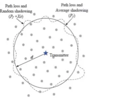
Fig. 2. The contour of RSS subject to path loss is a circle centered at the transmitter, and the contour of RSS attenuated by both path loss and shadowing is an irregular loop fluctuating around the path-loss circle.

In this section, we focus on formulating the evaluation feedback metric using collected JSS measurements. In particular, we model the jammer localization as an optimization problem. We delay the discussion of JSS measurement scheme MeasureJSS() to Section V and searching algorithms SearchForBetter() to Section VI.

1. Radio Propagation Basics

In wireless communication, the received signal strength attenuates with the increase of distance between the sender and receiver due to path loss and shadowing, as well as constructive and destructive addition of multipath signal components [8], [9]. Path loss can be considered as the

average attenuation while shadowing is the random attenuation caused by obstacles through absorption, reflections, scattering, and diffraction [8], [9]. Figure 2 illustrates contours of a received signal strength and the relationship between shadowing and path loss. The attenuation caused by shadowing at any single location, d meters from the transmitter, may exhibit variation; the average attenuation and average signal strength on the circle centered at the transmitter are roughly the same [8],[9]. This observation serves as the fundamental basis of our error minimizing framework. To illustrate our jammer localization approach, we use the widely-used log-normal shadowing model [8],[9], which captures the essential of both path loss and shadowing. Let Pf be the received signal strength subject to path loss attenuation only, and let the power of a transmitted signal be Pt. The received signal power in dBm at a distance of d can be modeled as the sum of Pf and a variance (denoted by Xσ) caused by shadowing and other random attenuation,

(1)

(2)

where Xσ is a Gaussian zero-mean random variable with standard deviation σ, K is a unit less constant which depends on the antenna characteristics and the average channel attenuation, and η is the Path Loss Exponent (PLE). In a free space, η is 2 and Xσ is always 0.

2. Localization Evaluation Metric

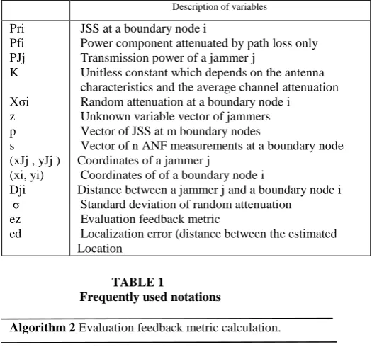
In this section, we discuss the definition of the evaluation metric , and we show the property of as well as its calculation. For the ease of reading, we summarize the frequently used notations in Table 1.

2.1 The property of

The definition of should have the following property: The larger the estimation errors of jammers‟ locations are, the larger is. We define as the estimated standard deviation of Xσ derived from the estimated jammers‟ locations. Considering the one jammer case, when the estimated jammer‟s location equals the true value, is the real standard deviation of Xσ, which is relatively small. When there is an estimation error (the estimated location is distance away from the true location), will be biased and will be larger than the real standard deviation of Xσ. The level of bias is affected by : the larger ed is, the bigger the estimated standard deviation of Xσ will likely be.The detailed relationship between and will be discussed in Section V.1.

one. Given the measured JSS, the estimated shadowing attenuation ( ) has to be larger than thereal one (Xσ1 ) to make up for the under-estimated . Similarly, and . Thus, the estimated shadowing attenuation { } exhibits a larger variance than the real one, and the estimated standard deviation ( ) corresponding to ( ) is larger than the true standard deviation. We note that the relationship between and is independent to the distribution of Xσ. Thus, in cases where the log-normal shadowing model does not match with the real radio propagation can still provide quantitative feedback of

2.2 Calculation

Single Jammer. Assume a jammer J located at ( ) starts to transmit at the power level of PJ, and m nodes located at {( )}i∈[1,m] become boundary nodes.To calculate , each boundary node will first measure JSS locally (the details will be discussed in Section V), and we

denote the JSS measured at boundary node i as . Let the current estimation of the jammer J‟s location and the transmission power be

̂ [ ̂ ̂ ̂ ̂]

Fig. 3. Illustration of jammer localization basis. When the estimated jammer location is meters from the true location, the estimated random attenuation is biased and the corresponding standard deviation is larger than the real one.

TABLE 1

Frequently used notations

Algorithm 2 Evaluation feedback metric calculation. 1: procedure EVALUATEMETRIC( ̂, p)

2: for all i ∈ [1,m] do

3: ̂ ̂ 4: end for

5: √ ∑ ̂ ̅̅̅̅̂

6: end procedure

Given ̂ we can estimate , the JSS subject to path loss only at boundary node i as

(̂ ) =̂ + ̂− 10η log10 ( ̂) (3)

̂ ̂ = √ ̂ ̂

Description of variables

Pri Pfi PJj K

Xσi z p s (xJj , yJj ) (xi, yi) Dji σ ez ed

JSS at a boundary node i

Power component attenuated by path loss only Transmission power of a jammer j

Unitless constant which depends on the antenna characteristics and the average channel attenuation Random attenuation at a boundary node i

Unknown variable vector of jammers Vector of JSS at m boundary nodes

Vector of n ANF measurements at a boundary node Coordinates of a jammer j

Coordinates of of a boundary node i

Distance between a jammer j and a boundary node i Standard deviation of random attenuation

Evaluation feedback metric

The random attenuation (shadowing) between the jammer J and boundary node i can be estimated as

̂ ̂ (4)

The evaluation feedback metric for the estimation ˆz is the standard deviation of estimated { ̂ }i∈[1,m],

̂ √ ∑ ̂ ̅̅̅̅̂ (5)

where ̅̅̅̅̂ is the mean of ̂ .One of the biggest advantages of this definition is that by subtracting ̅̅̅̅, is only affected by (̂ ̂) and is independent of the estimated jamming power ̂ ̂.

Algorithm 3 Acquiring the Ambient Noise Floor

(ANF). ANF approximates the strength of jamming signals.

1: procedure MEASUREJSS 2: s = {s1, s2, ..., sn} = MeasureRSS() 3: if var(s) < varianceThresh then

4: sa = s

5: else

6: JssThresh = min(s) + α[max(s) − min(s)] α ∈ [0, 1] 7: = { < JssThresh, ∈s }

8: end if

9: return mean( ) 10: end procedure

Multiple Jammers. Similar to single jammer, we assume n jammers located at {( )}i∈[1,n] start to transmit at the power level of { }i∈[1,n] separately at the same time, and m nodes located at {(xi, yi)}i∈[1,m] become boundary nodes.To calculate , each boundary node measures JSS locally and we denote the JSS measured at boundary node i as which is a combined JSS from multiple jammers. We can include all the variables to be estimated, i.e., current estimation of the n jammers‟ locations and the transmission powers, in a form of matrix written as

In the case of multiple jammers, pfi is the combined JSS from n jammers subject to path loss at a boundary node and can be calculated as

̂ =10 ∑

̂ ̂

̂

(7)

̂=√ ̂ ̂

where ̂ is the estimated distance between jammer j and boundary node i.Note that ̂ , ̂ and are all in dBm. Then, the random attenuation between multiple jammers and the boundary node i can be estimated as

̂ , (8)

Thus, the evaluation feedback metric of ̂is

̂ =√ ∑ ̂ ̅̅̅̅̂

where ̅̅̅̅̂is the mean of ̂ . 2.3 Problem Formulation.

Given the definition of the feedback metric ( ), we generalize jammer localization problem as one optimization problem,

Problem 1:

Minimize (z, p)

z

where z are the unknown variable matrix of the jammer( s), e.g., z is defined in Eq. (6), and { }i∈[1,m] are the JSS measured at the boundary nodes {1, . . .,m}. As we will show in Section V.1, the estimated location(s) of the jammer(s) at which is minimized, matches the true location(s) of jammer(s) with small estimation error(s).

V.

M

J

S

Received signal strength (RSS) is one of the most widely used measurements in localization. For instance, a WiFi device can estimate its most likely location by matching the measured RSS vector of a set of WiFi APs with pre-trained RF fingerprinting maps [10] or with predicted RSS maps constructed based on RF propagation models [11]. However, obtaining signal strength of jammers (JSS) is a challenging task mainly because jamming signals are embedded in signals transmitted by regular wireless devices. The situation is complicated because multiple wireless devices are likely to send packets at the same time, as jamming disturbs the regular operation of carrier sensing multiple access (CSMA). For the rest of this paper, we refer the regular nodes‟ concurrent packet transmissions that could not be decoded as a collision While it is difficult, if ever possible, to extract signal components contributed by jammers or collision sources, we discover that it is feasible to derive the JSS based on periodic ambient noise measurement. In the following subsections, we first present basics of ambient noise with regard to jamming signals, and then introduce our scheme to estimate the JSS. Finally, we validate our estimation schemes via real-world experiments.

1. Basics of Ambient Noise Floor

In theory, ambient noise is the sum of all unwanted signals that are always present, and the ambient noise floor (ANF) is the measurement of the ambient noise. In the presence of constant jammers, the ambient noise includes thermal noise, atmospheric noise, and jamming signals. Thus, it is

PN = PJ + PW, (10)

where PJ is the JSS, and PW is the white noise comprising thermal noise, atmospheric noise, etc. Realizing that at each boundary node PW is relatively small compared to PJ , the ambient noise floor can be roughly considered as JSS. Thus, estimating JSS is equivalent to deriving the ambient noise floor (ANF) at each boundary node. In this work, we consider the type of wireless devices that are able to sample ambient noise regardless of whether the communication channel is idle or busy, e.g., MicaZ sensor platforms; and derive the ANF based on ambient noise measurements.

A naive approach of estimating the ANF could be sampling ambient noise when the wireless radio is idle (i.e., neither receiving nor transmitting packets). Such a method may not work in all network scenarios, since it may result in an overestimated ANF. For example, in a highly congested network, collision is likely to occur, and the collided signals may be treated as part of the ANF at the receiver, resulting in an inflated ANF. This is exactly the situation we want to avoid.

2. Estimating Strength of Jamming Signals

To derive the JSS, our scheme involves sampling ambient noise values regardless of whether the channel is idle or busy. In particular, each node will sample n measurements of ambient noise at a constant rate, and denote them as s = [s1, s2, . . . , sn]. The measurement set s can be divided into two subsets (s = ∪ ).

1) = { = PJ}, the ambient noise floor set that contains the ambient noise measurements when only jammers are active, and 2) = { = }, the combined ambient noise set that contains ambient noise measurements when both jamming signals (PJ )

and signals from one or more senders (PC) are present.

Calculating JSS is equivalent to obtaining the average of ANFs, i.e., mean(sa). In most cases, ≠∅ and ⊂s. In a special case where no sender has ever transmitted packets throughout the process of obtaining n measurements, = ∅ and = s. The algorithm for calculating the ANF should be able to cope with both cases. As such, we designed an algorithm (referred as Algorithm 3) as follows: A regular node will take n measurements of the ambient noise measurements. It will consider the ANF as the average of all measurements if no sender has transmitted during the period of measuring; otherwise, the ANF is the average of sa, which can be obtained by filtering out sc from s. The intuition of differentiating those two cases is that if only jamming signals are present, then the variance of n measurements will be small; otherwise, the ambient noise measurements will vary as different senders happen to transmit.

The correctness of the algorithm is supported by the fact that is not likely to be empty due to carrier sensing, and the JSS approximately equals to the average of .The key question is how to obtain . To do so, we set the upper bound (i.e., JssThresh) of sc in Algorithm 3 as α percentage of the amplitude span of ambient noise measurements. We validate the feasibility of obtaining using a filtering bound in the next experimental subsection.

VI. ALGORITHM DESCRIPTION

1. A Genetic Algorithm

A genetic algorithms (GA) [12] searches for the global optimum by mimicking the process of natural selection in biological evolution. A GA iteratively generates a set of solutions known as a population. At each iteration, a GA selects a subset of solutions to form a new population based on their “fitness” and also randomly generates a few new solutions. As a result, the “fitter” solutions will be inherited. At the same time, new solutions will be introduced to the population, which may turn out to be “fitter” than ever. As a result, over successive generations, a GA is likely to escape from local optima and “evolves” towards an optimal solution.

VII.

C

R

In this paper, deliberatively finding the issues to minimize the errors while localizing a jammer in wireless networks .The jamming is a wireless device which is used to produce unintentionally interference of radio or maliciously defined jammer which is troubling the network. For reducing the estimated error, further designing a survey on error minimizing based framework for focusing on the jammer.Outlining an evaluated feedback metric which quantifying the estimated error of jammer‟s position and analyzing the affiliation between the evaluated feedback metric and estimated errors. And also increasing the estimated accuracy by designing an error which minimizes framework to localize jammers .Using this method it can increase the efficiency, packet delivery ratio and decreasing the packet loss, energy spent and delay.

R

[1] K. Pelechrinis, I. Koutsopoulos, I. Broustis, and S. V. Krishnamurthy, “Lightweight jammer localization in wireless networks: System design and implementation,” in Proceedings of IEEE GLOBECOM, 2009.

[2] H. Liu, Z. Liu, Y. Chen, and W. Xu, “Determining the position of a jammer using a virtual-force iterative approach,” WirelessNetworks (WiNet), vol. 17, pp. 531–547, 2010.

[3] Z. Liu, H. Liu, W. Xu, and Y. Chen, “Exploiting neighbor changes for jammer localization,” IEEE TPDS, vol. 23, no. 3, 2011. [4] H. Liu, Z. Liu, Y. Chen, and W. Xu, “Localizing multiple jamming attackers in wireless networks,” in Proceedings ofICDCS, 2011. [5] T. Cheng, P. Li, and S. Zhu, “Multi-jammer localization in wireless sensor networks,” in Proceedings of CIS, 2011.

[6] A. Wood, J. Stankovic, and S. Son, “JAM: A jammed-area mapping service for sensor networks,” in Proceedings of RTSS.

[7] W. Xu, W. Trappe, Y. Zhang, and T. Wood, “The feasibility of launching and detecting jamming attacks in wireless networks,” in Proceedings of MobiHoc, 2005.

[8] A. Goldsmith, Wireless Communications. Cambridge University Press, 2005. [9] T. Rappaport, Wireless Communications- Principles and Practice. Prentice Hall, 2001.

[10] P. Bahl and V. N. Padmanabhan, “RADAR: An in-building RF-based user location and tracking system,” in Proceedings ofINFOCOM, 2000.

[11] J. Yang, Y. Chen, and J. Cheng, “Improving localization accuracy of rss-based lateration methods in indoor environments,” AHSWN, vol. 11, no. 3-4, pp. 307–329, 2011.

[12] D. Goldberg, Genetic algorithms in search, optimization and machine learning. Addison-Wesley, 1989. [13] E. Polak, Computational Methods in Optimization: a Unified Approach. Academic Press, 1971. [14] P. V. Laarhoven and E. Aarts, Simulated Annealing: Theory and Applications. Springer, 1987.

[15] Z. Liu, H. Liu, W. Xu, and Y. Chen, “Wireless jamming localization by exploiting nodes‟ hearing ranges,” in Proceedings ofDCOSS,2010. [16] Y. Chen, J. Francisco, W. Trappe, and R. P. Martin. A practical approach to landmark deployment for indoor localization. In SECON, 2006. [17] A. Goldsmith. Wireless Communications. Cambridge University Press, 2005.

[18] S. Khattab, D. Mosse, and R. Melhem. Modeling of the channel-hopping anti-jamming defense in multi-radio wireless networks. In Proceedings of Annual International Conference on Mobile and Ubiquitous Systems,pages 1–10, 2008.

[19] K. Ma, Y. Zhang, and W. Trappe. Mobile network management and robust spatial retreats via network dynamics. In Proceedings of International Workshop on Resource Provisioning and Management in Sensor Networks, 2005.

[20] V. Navda, A. Bohra, S. Ganguly, R. Izmailov, and D. Rubenstein. Using channel hopping to increase 802.11 resilience to jamming attacks. In IEEE Infocom Minisymposium, pages 2526 – 2530, 2007.

[21] G. Noubir and G. Lin. Low-power DoS attacks in data wireless LANs and countermeasures. Mobile Computting Communications Review, 7(3):29–30, 2003. [22] N. Priyantha, A. Chakraborty, and H. Balakrishnan. The cricket location support system. In MobiCom, pages 32–43, 2000.

[23] Y. Sun and X. Wang. Jammer localization in wireless sensor networks. In Proceedings of International Conference on Wireless communications, networking and mobile computing, pages 3113–3116, 2009.

[24] R. Want, A. Hopper, V. Falcao, and J. Gibbons. The active badge location system. ACM Transactions on Information Systems, 10(1):91– 102, 1992. [25] A. Ward, A. Jones, and A. Hopper. A new location technique for the active office. IEEE Personal Communications, 4(5):42–47, 1997.

[26] W. Xu, W. Trappe, and Y. Zhang. Channel surfing: defending wireless sensor networks from interference. In Proceedings of International conference on Information processing in sensor networks, pages 499– 508, 2007.