Diffraction by a Wedge or by a Cone with Impedance-Type Boundary Conditions and Second-Order Functional Difference Equations

DIFFRACTION BY A WEDGE OR BY A CONE WITH IMPEDANCE-TYPE BOUNDARY CONDITIONS AND SECOND-ORDER FUNCTIONAL DIFFERENCE

EQUATIONS N. Y. Zhu

Institut f¨ur Hochfrequenztechnik Universit¨at Stuttgart

Pfaffenwaldring 47, D-70550 Stuttgart, Germany

M. A. Lyalinov

Department of Mathematical Physics Institute of Physics

St. Petersburg University

Ul’yanovskaya 1-1, Petrodvorets-St. Petersburg, 198904, Russia Abstract—This work reports some recent advances in diffraction theory by canonical shapes like wedges or cones with impedance-type boundary conditions. Our basic aim in the present paper is to demonstrate that functional difference equations of the second order deliver a very natural and efficient tool to study such a kind of problems.† To this end we consider two problems: diffraction of a normally incident plane electromagnetic wave by an impedance wedge whose exterior is divided into two parts by a semi-infinite impedance sheet and diffraction of a plane acoustic wave by a right-circular impedance cone. In both cases the problems can be formulated in a traditional fashion as boundary-value problems of the scattering theory.

For the first problem the Sommerfeld-Malyuzhinets technique enables one to reduce it to a problem for a vectorial system of functional Malyuzhinets equations. Then the system is transformed to uncoupled second-order functional difference-equations (SOFDE) for each of the unknown spectra. In the second problem the incomplete separation of variables leads directly to a functional difference-equation of the second order. Hence, it is remarkable that in both cases the key

† _{For a thorough and up-to-date overview of the scattering and diffraction in general the}

mathematical tool is an SOFDE which is an analog of a second-order differential equation with variable coefficients. The latter is reducible to an integral equation which is known to be the most traditional tool for its solution. It has recently been recognised that reducing SOFDEs to integral equations is also one of the most efficient approaches for their study.

The integral equations which are developed for the problems at hand are both of the second kind and obey Fredholm property. In the problem of diffraction by a wedge the generalised Malyuzhinets function is exploited on the preliminary step then “inversion” of a simple difference operator with constant coefficients leads to an integral equation of the second kind. The corresponding integral operator is represented as a sum of the identical operator and a compact one [2]. However, in the second problem the situation is slightly different: the integral operator can be represented by a sum of the boundedly-invertible (Dixon’s operator) and compact operators. This situation was earlier considered by Bernard in his study of diffraction by an impedance cone, and important advances have been made (see [3–6]). The Fredholm property is crucial for the elaboration of different numerical schemes. In our cases we exploited direct numerical approaches based on the quadrature formulae and computed the far-field asymptotics for the problems at hand. Various numerical results are demonstrated and discussed.

1. DIFFRACTION BY AN IMPEDANCE WEDGE WITH A SEMI-INFINITE IMPEDANCE SHEET ATTACHED TO ITS EDGE

method. From evaluation of the Sommerfeld integrals by virtue of the saddle-point method a first-order uniform asymptotic solution follows. The results to be given below follow the same line as [2, 7]. Therefore, the following exposition is confined to main steps and the readers are referred to [2, 7] for details.

1.1. Statement of the Problem

Figure 1 depicts the scattering obstacle. For convenience, a cylindrical co-ordinate system (r, ϕ, z) is chosen in such a way that the edge of the wedge and one rim of the semi-infinite impedance sheet coincide with the z-axis, the wedge faces and the impedance sheet are half-planes given by ϕ=±Φ and ϕ= Φ0 with 0<Φ≤π. In the following, it is assumed that 0≥Φ0≥ −Φ.

Figure 1. Diffraction of a normally incident plane wave in a wedge-shaped region.

A plane wave impinges perpendicularly on the edge from the direction ϕ = ϕ0 with Φ0 < ϕ0 < Φ assumed in this study. The alternative case can be dealt with analogously. The incident electric field oscillates along the edge of the wedge-shaped region and is given by (a time-dependence e−iωt is assumed and suppresed in this section)

This incident wave will be scattered by the obstacle. Owing to the translational symmetry of both the incident wave and the wedge-shaped region with respect to thez-axis, the boundary value problem is a two-dimensional one and the total electric field has only one component Ez(r, ϕ).

In the region surrounding the wedge and the sheet, Ez obeys

the two-dimensional Helmholtz equation. On the faces of the wedge

ϕ=±Φ, the boundary conditions to be met by Ez read

1

r ∂

∂ϕEz∓i k

η_±Ez = 0, (2)

η_±Z0 being the surface impedance of the upper (lower) wedge face and

Z0 the intrinsic impedance of the surrounding medium.

The electric property of the impedance sheet is given byys/Z0, the shunt admittance. On the impedance sheet atϕ= Φ0,Ez is subjected

to the semi-transparency conditions [8]:

1

r ∂ ∂ϕEz

+

−

1

r ∂ ∂ϕEz

₋

+ ikys

2[E +

z +Ez−] = 0,

[E_z+−E_z−] = 0.

(3)

Furthermore,Ez must satisfy the Meixner’s edge conditionEz = O(1)

asr→0 and the radiation conditions [9] (see also [10]). 1.2. Higher-Order Functional Difference-Equation

According to Sommerfeld, the solution can be constructed through a superposition of plane waves

Ez = E0 2πi

γ

S_±(α+ϕ) exp(−ikrcosα) dα, ϕ∈

[Φ0,Φ]

[−Φ,Φ0] (4)

γ denotes the Sommerfeld double loops (see [9, 10]). S_±(α) are the complex spectra of the electric field Ez in the angular regions above

and below the impedance sheet.

Inserting the above expressions forEz into (2) and (3) and then

inverting the Sommerfeld integrals, we obtain a coupled system of Malyuzhinets equations

(sinα±sinϑ_±)S_±(α±Φ) = (−sinα±sinϑ_±)S_±(−α±Φ), (5) (sinα−sinϑ)[S+(α+ Φ0)−S−(−α+ Φ0)]

= (sinα+ sinϑ)[S₋(α+ Φ0)−S+(−α+ Φ0)], (6)

Complex angles ϑand ϑ_± have been introduced according to sinϑ=ys/2, 0≤Reϑ≤π/2; sinϑ±=η_±−1, 0≤Reϑ±≤π/2.

To satisfy the radiation conditions we demand

S+(α)−1/(α−ϕ0) be regular in Π(Φ0,Φ), S₋(α) be regular in Π(−Φ,Φ0).

(8)

The presence of a pole at the point α=ϕ0 for the functionS+ serves to recover the incident plane wave. And the Meixner’s condition determines the asymptotic behaviour of the spectral functions:

S_±(α) = O(1) as α→ ±i∞.

By eliminatingS₋ from (5)–(7) we arrive at a difference-equation forS+ alone

−

1 +sinϑ sinα

S+(α−Φ0+ 2Φ)

R+(α−Φ0+ Φ) +

1− sinϑ sin(α−2Φ0−2Φ)

×R₋(α−Φ0−Φ)S+(α−Φ0−2Φ) = sinϑ

sinαS+(α+ Φ0)

+ sinϑ sin(α−2Φ0−2Φ)

R₋(α−Φ0−Φ)

R+(α−3Φ0−Φ)

S+(α−3Φ0). (9) where R_±(α) = (sinα − sinϑ_±)/(sinα + sinϑ_±) is the reflection coefficient of the upper (lower) wedge face. Apparently, the poles in the basic strip Π(−2Φ,2Φ) and their principal parts are

S+(α) = 1/(α−ϕ0) +. . . ,

S+(α) = H(Φ + 2Φ0−ϕ0)R(ϕ0−Φ0)/[α−(2Φ0−ϕ0)] +. . . andR(ϕ) =−sinϑ/(sinϑ+sinϕ) means the reflection coefficient of the impedance sheet. As usual,H(·) is the Heaviside unit step function.

Unlike the functional difference-equations encountered in our previous works [2, 7], Equation (9) is of higher order and reduces to an equation of the second order merely for Φ0 = 0. Despite this difference, the technique developed in [2, 7] can be applied to solving (9).

1.3. Simplified Functional Difference-Equation

Let us construct an even function now and begin with the boundary condition on the upper wedge face, see (5). By making use of a generalised Malyuzhinets function χΦ which obeys a first-order functional difference-equation and is specially normalised

χΦ(α+ 2Φ)

χΦ(α−2Φ) = cos

α

2

and its relationship to the well-known Malyuzhinets function

ψΦ [2, 8, 11–13]

ψΦ(α) = 1 [χΦ(π/2)]2

χΦ(α+π/2)

χΦ(α−π/2)

, (11)

we come to the conclusion that (5) is equivalent to

S+(α+ Φ)/Ψ+(α+ Φ) =S+(−α+ Φ)/Ψ+(−α+ Φ), with Ψ_±(α) =ψΦ(α+ϑ±±Φ−π/2)ψΦ(α−ϑ±±Φ +π/2).

Therefore, the looked-for even functionψ(α) is defined as

ψ(α) =S+(α+ Φ)/Ψ+(α+ Φ). (12) Its principal parts at two polesα=−Φ + 2Φ0−ϕ0 and α=−Φ +ϕ0 located in the strip Π(−2Φ,0) are known

ψ(α) = H(Φ + 2Φ0−ϕ0)R(ϕ0−Φ0) [α+ (Φ−2Φ0+ϕ0)] Ψ+(2Φ0−ϕ0)

+· · ·,

ψ(α) = 1

[α+ (Φ−ϕ0)] Ψ+(ϕ0)

+· · · .

(13)

In view of the evenness of ψ(α) the other two poles in the strip Π(−2Φ,2Φ) and their principal parts are also known. From (9) follows the governing equation forψ(α). Introduce once again a new function

F(α) via ψ(α) = χ(α)F(α) where χ(α) must be even and regular in the basic strip and furthermore meet the following first order difference equation

χ(α+2Φ)

χ(α−2Φ)=−

sin(α−Φ0−Φ)−sinϑ sin(α+Φ0+Φ)+sinϑ

sin(α+ Φ0+ Φ)

sin(α−Φ0−Φ)R−(α). (14) By virtue of (10) and (11), an appropriateχ(α) with all the necessary properties is found to be (cf. [2, 7])

χ(α) = χΦ(α−Φ0−Φ−ϑ+π)χΦ(α−Φ0−Φ +ϑ)

χΦ(α+ Φ0+ Φ +ϑ−π)χΦ(α+ Φ0+ Φ−ϑ)

×χΦ(α+ Φ0+ Φ−π)χΦ(α+ Φ0+ Φ) χΦ(α−Φ0−Φ +π)χΦ(α−Φ0−Φ)

Ψ₋(α+ Φ).

The asymptotic behaviours ofχΦ(α) and ψΦ(α) dictate that of χ(α):

χ(α) = O(e∓iµα/2) as Imα → ±∞. Here, µ = π/(2Φ). Therefore,

Using F(α) in place of ψ(α) in the governing equation for the latter and making use of (14), one gets the following simple difference equation for F(α)

F(α+2Φ)−F(α−2Φ) =Q1(α)F(α+ 2Φ0)+Q2(α)F(α−2Φ0), Q1(α) =−R(α+ Φ0+ Φ)

χ(α+ 2Φ0)

χ(α+ 2Φ)

Ψ+(α+ 2Φ0+ Φ) Ψ+(α−Φ) ,

Q2(α) =−R(α+ Φ0+ Φ)χ(α−2Φ0)

χ(α+ 2Φ)

Ψ+(α−2Φ0+ Φ) Ψ+(α−Φ)

×sin(α+ Φ0+ Φ) sin(α−Φ0−Φ)

R₋(α)

R+(α−2Φ0)

.

(15)

Q1andQ2are related to each other: Q1(−α) =−Q2(α), therefore, the right-hand side of the FDequation for F(α) is odd. In addition, the asymptotic behaviour ofQ1 and Q2 is found to be Q1,2(α) = O(e±iα) as Imα→ ±∞.

1.4. Fredholm Integral Equation of the Second Kind

It follows from the evenness of F(α) and the relation between Q1(α) and Q2(α) that (15) amounts to

F(α±2Φ)−F(−α±2Φ) =±[Q1(α)F(α+ 2Φ0) +Q2(α)F(α−2Φ0)].

Considering the right-hand sides of the latter equations as inhomo-geneity terms, the solution of the above equations contains the general solution of the homogeneous equations and the particular solution of the inhomogeneous equations. If the right-hand side of (15), an odd function of the order e±iα(1+µ)_{as Imα→ ±∞, is known, the particular} solution can be constructed using the so-called S-integrals [8, 10, 14]. This way is comparable to utilising a modified Fourier transform with integration along the imaginary axis. Hence we have an integral equiv-alent to (15), namely

F(α) = C1µcos(µϕ0) cos(µα)−sin(µϕ0) + C2µcos[µ(ϕ0−2Φ0)]

cos(µα) + sin[µ(ϕ0−2Φ0)]

H(Φ + 2Φ0−ϕ0)

+ i 4Φ

_i∞

−i∞

Q1(t) sin(µt)F(t+ 2Φ0) dt

2Φ0 + ϕ0) in the basic strip Π(−2Φ,2Φ) with known principal parts. Therefore, C1 = 1/[χ(Φ−ϕ0)Ψ+(ϕ0)], C2 = R(ϕ0 − Φ0)/[χ(Φ−2Φ0+ϕ0)Ψ+(2Φ0−ϕ0)].

Because (16) is valid for every point α inside the basic strip Π(−2Φ,2Φ) of the complex plane, it also remains true for points on a shifted imaginary axis Reα= 2Φ0. Exactly for this shifted imaginary axis, (16) becomes a Fredholm integral equation of the second kind. A brief discussion on how to solve this integral equation numerically will be given in the next subsection.

Having found the numerical value for F(α) along the shifted imaginary axis Reα= 2Φ0, (16) is used to calculateF(α) and therefore

S+(α) inside the basic strip Π(−2Φ,2Φ) and analytical extension where necessary. S₋(α), the other spectral function, is determined through its relation to S+(α)

S₋(α) =

1− sinϑ sin(α−Φ0)

S+(α) + sinϑ sin(α−Φ0)

S+(−α+ 2Φ0). (17) Evaluating asymptotically the Sommerfeld integrals yields a first-order uniform asymptotic solution which is of particular interest:

Ez(r, ϕ)∼Ezgo(r, ϕ) +Ezd(r, ϕ) +Ezsw(r, ϕ). (18)

As usual, the super indices “go”, “d”, and “sw” signify geometrical-optics, diffracted, and surface-wave parts. Especially, there is

E_zd(r, ϕ) = exp (i√ kr)

r D±(r, ϕ)E0, ϕ∈

[Φ0,Φ] [−Φ,Φ0]

where D_±(r, ϕ) denotes the uniform diffraction coefficient of such a canonical structure (see for instance [2]).

1.5. Verificationand Numerical Solution

the generalised Malyuzhinets function χΦ, we resort to a procedure described in detail in [13].

It is worth mentioning that the solution described above reduces both analytically and numerically to the one given in [7] in which the semi-infinite impedance sheet bisects the exterior of the impedance wedge, that is Φ0= 0.

Also a 90◦ angle formed by a perfectly conducting half-plane and a semi-infinite impedance sheet can be studied. Fig. 2 displays the amplitude of the total electric field on a circle of radiuskr= 12 centred on the edge, together with the results obtained in [15] by means of an approximate procedure, the parabolic equation method. Away from the impedance sheet located atϕ= Φ0 =−90◦, the two results agree very well, confirming additionally the present work and furthermore demonstrating the surprisingly high accuracy of the parabolic equation method.

-180 -150 -120 -90 -60 -30 0 30 60 90 120 150 180

ϕ(degrees)

0 0.2 0.4 0.6 0.8 1 1.2 1.4 1.6 1.8 2

|E

(r

,

ϕ

)|

(V

/m

)

This work PEM

ϑ±

=π/2+i∞, ϑ= 0.02477-i0.5254,

Φ=π, Φ0= -π/2, k0r = 12, ϕ0= -π/3

2. ACOUSTIC SCATTERING OF A PLANE WAVE BY A RIGHT-CIRCULAR IMPEDANCE CONE

The analytic solution is constructed on the basis of the incomplete separation of variables and of reduction to a problem for a second-order functional difference-equation (SOFDE). Though the latter is equivalent to a Carleman boundary-value problem for analytic vectors, the solution is sought for by means of the direct reduction converting the SOFDE to a Fredholm-type integral equation. Its unique solvability will be then studied and the expression for the scattering amplitude of the spherical wave from the vertex be discussed. This section is based on [3, 4, 6, 16]. We note that a similar analysis is presented in [5] in which numerical results for axial incidence are given and therefore, will be called upon for comparison purposes. 2.1. Statement of the Problem

In the spherical coordinates (r, θ, ϕ) which are related to the Cartesian ones (x1, x2, x3) via

x1 = rsinθ cosϕ, x2 = rsinθ sinϕ, x3 = rcosθ, (19) the axis Ox3 coincides with the axis of the right-circular impedance cone under study, where θ = θ1 is the equation of the cone’s surface withπ/2< θ1 < π(Fig. 3).

The incident plane wave field in the spherical coordinates is given by

Ui = e−ikrcos ˆθ(ω,ω0)_{, k = Ω/c . (20)}

where ω0 = (θ0, ϕ0) is the unit vector attached to the direction of incidence, ω = $r/r = (θ, ϕ), cos ˆθ(ω, ω0) = cosθcosθ0 + sinθsinθ0cos(ϕ−ϕ0), c is the wave speed in the acoustic medium. The harmonic dependence on time e−iΩt _{is omitted throughout this}

section. We assume also that the incident wave illuminates completely the conical surface from the exterior that isθ0< π−θ1.‡

The scattered acoustic fieldU satisfies the Helmholtz equation

+k2U = 0, (21)

and the boundary conditions 1

r

∂U +Ui ∂θ

θ=θ1

− ikη U+Ui θ=θ1

= 0, (22)

‡ _{The procedure given here can equally be used to study the case of a partly-lit impedance}

O 1 x2

x3

0 r

1

n

θ

θ

ϕ

x

θ

η

Figure 3. Diffraction of an acoustic plane wave by a right-circular impedance cone.

as well as the Meixner’s condition at the tip of the cone and the condition at infinity. See [3–6, 16].

2.2. Incomplete Separation of Variables

The scattered acoustic fieldU is sought in the form of the Kontorovich-Lebedev integral [3, 4, 6, 16]

U(kr, ω, ω0) = 4 i√2π

_i∞

−i∞

νsin(πν)uν(ω, ω0)

K_√ν(−ikr)

−ikr dν , (23)

whereω= (θ, ϕ) denotes the direction of scattering andω0specifies the direction of incidence. Kν(·) stands for the modified Bessel function

uν(ω, ω0) by dint of a Fourier expansion in azimuth ϕ:

uν(ω, ω0) =

+∞

n=_−∞

ine−inϕRu(ν, n)

P_ν−|₋n_1/|₂(cosθ) dθ1P

−|n|

ν−1/2(cosθ1)

, (24)

where P_ν−|₋n₁|_/2(cosθ) is a Legendre function. In a similar fashion, the incident field Ui is also expressed in the form of the Kontorovich-Lebedev integral

Ui(kr, ω, ω0) = 4 i√2π

i∞

−i_∞

νsin(πν)ui_ν(ω, ω0)

K_√ν(−ikr)

−ikr dν (25)

whereui_ν(ω, ω0) is given by

ui_ν(ω, ω0) = +∞

n=_−∞

ine−inϕRi(ν, n) P

−|n_|

ν−1/2(−cosθ) dθ1P

−|n|

ν−1/2(−cosθ1)

(26)

with

Ri(ν, n) = i

n

−4 cos(πν)

Γ(ν+|n|+ 1/2) Γ(ν− |n|+ 1/2)

×dθ1P −|n|

ν−1/2(−cosθ1)P

−|n|

ν−1/2(cosθ0).

Inserting the above expressions for the scattered field and the incident field in the boundary condition on the cone’s surface (22) and inverting the integrals, we arrive at the governing relation for the unknownRu(ν, n) :

Ru(ν+ 1, n)−Ru(ν−1, n) =−2i ηw(ν, n)Ru(ν, n) +S(ν, n), (27)

which is a second-order functional difference-equation (SOFDE).w, S

are known meromorphic function ofν:

S(ν, n) = −[Ri(ν+ 1, n)−Ri(ν−1, n)]−2i ηwi(ν, n)Ri(ν, n),

w(ν, n) = −iν P −|n_|

ν−1/2(cosθ1) dθ1P

−|n|

ν−1/2(cosθ1)

,

wi(ν, n) = −iν

P_ν−|₋n₁|_/2(−cosθ1) dθ1P

−|n|

ν−1/2(−cosθ1)

.

2.3. Reductionto a Fredholm Integral Equation

As in the first problem for a wedge the SOFDE (27) is reduced to a integral equation of the second kind§

Ru(ν, n) = η _i∞

0

w(t, n)Ru(t, n) sin(πt)

cos(πt) + cos(πν) dt + Si(ν, n). (28) with

Si(ν, n) =−Ri(ν, n) +η

_i∞

0

wi(t, n)Ri(t, n) sin(πt) cos(πt) + cos(πν) dt. Having obtained Ru(t, n) as t ∈iR, this function is then analytically

continued as a meromorphic function. A remarkable property of the integral equation (28) is that its solution is unique (Reη > 0) in the respective class of functions. We demonstrate subsequently that the integral equation possesses the Fredholm property (its operator can be represented as a sum of boundedly-invertible and compact operators) then its solvability follows from uniqueness, which is a standard trick for this kind of equations. This equation is to be solved by use of numerical methods.

Replacing in the Kontorovich-Lebedev integral (23) the Macdon-ald function by its approximate expression for large arguments, the scattered acoustic pressureU in “oasis”, i.e., in the domain not illumi-nated by the reflected rays, has the asymptotics

U(kr, ω, ω0) =D(ω, ω0) e ikr

−ikr

1 + O

1

kr

, (29)

where

D(ω, ω0) = 2 i

_i∞

−i∞

νsin(πν)uν(ω, ω0) dν (30)

is the scattering diagram (amplitude) or diffraction coefficient. It is noted that the asymptotics (29) is valid solely inside the oasis, hence non-uniform.

2.4. Perturbative Solutionof the SOFDE

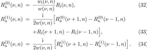
In case of large or small amplitude of the impedanceη, a perturbative solution of the functional difference-equation (27) can be constructed. For example, for large|η| the following series for Ru(ν, n) seems

feasible

Ru(ν, n) =R(0)u (ν, n) +η−1R(1)u (ν, n) +η−2R(2)u (ν, n) +. . . (31)

Inserting the above Ansatz in the SOFDE for Ru(ν, n) and equating

the coefficients of like powers ofη we get

R(0)_u (ν, n) = −wi(ν, n)

w(ν, n)Ri(ν, n), (32)

R(1)_u (ν, n) = i 2w(ν, n)

R(0)_u (ν+ 1, n)−R(0)_u (ν−1, n) +Ri(ν+ 1, n)−Ri(ν−1, n)

, (33)

R(2)_u (ν, n) = i 2w(ν, n)

R(1)_u (ν+ 1, n)−R_u(1)(ν−1, n)

. (34)

Clearly, the zeroth-order term R(0)u (ν, n) represents the exact solution

of (27) for an acoustically soft cone, whereas the first-order and higher-order terms refine the approximate solution to the functional difference-equation (27) for large but finite|η|.

The perturbative solution of (27) for small|η|can be deduced in a similar way.

2.5. Numerical Aspects and Examples

As implied by the above formulae, the determination of the diffraction coefficient (scattering diagram) Dfor a right-circular impedance cone consists of solving at first the integral equation (28) for each Ru(ν, n)

and then carrying out the integration along the imaginary axis of the

ν plane (29).

Also for the cone problem we take into account the known asymptotic behaviour of Ru(ν, n). The infinitely large interval is

transformed into a finite one via

ν = ip

θ1−θ0

ln1−ξ

1 +ξ, p1.

The Gauß-Legendre scheme is used in the numerical solution of the integral equation (28). For the integration contained in the diffraction diagram Dit proves beneficial to employ the Gauß-Laguerre scheme.

The first example in this Section concerns the axisymmetric case (the plane wave is incident along the axis of the cone θ0 = 0). Fig. 4 displays the amplitude of the diffraction coefficient |D(ω, ω0)| as a function of both the surface impedance η and the co-latitude

singular directions the far field is described by the parabolic cylinder functions (see for instance [6]).

Shown in Fig. 4 as symbols are the data obtained in [5] which corroborate our results.

0 50 100

θ(degree)

10-1 100

|D

(

ω

,

ω0

)|

η= 1010 η= 1 η= 0 Antipov

θ1= 150 o_{, θ}

0= 0 o

Figure 4. Diffraction by a right-circular impedance cone at axial incidence. Comparison with the results of Antipov [5].

At non-axial incidence, the diffraction coefficientD(ω, ω0) depends in addition upon the azimuth ϕ. This is also true for the singular direction θs(ϕ) with its smallest value occurring at ϕ =ϕ0; θs(ϕ0) = 2θ1−θ0−πand its maximum value attained atϕ=ϕ0±π :θs(ϕ0±π) = 2θ1+θ0−π. This fact explains the tilted contours shown in Fig. 5.

Displayed in Fig. 5 are also results based on the first two terms of the perturbation series (31).

3. EPILOGUE

In this paper we have reported some of our recent works on diffraction of waves by bodies of canonical shape: scattering of a normally incident plane electromagnetic wave by a semi-infinite impedance sheet attached to an impedance wedge and scattering of a non-axially incident plane acoustic wave by a right-circular impedance cone.

0 30 60 90 120 150 180 ϕ(degree) 0 20 40 60 80 100 θ (d e g re e ) 0.2 0.2 0.3 0.3 0.4 0.4 0.5 0.5 0.6 0.6 0.7 0.7 0.8 0.9 0.9 1 1.1 1.1 1.15 1.25 1.35 1.45 1.55 1.651.75 1.85 1.95 2.15 2.45 0.2 0.2 0.2 .3 0.3 0.3 0.4 0.4 0.4 0.5 0.5 0.6 0.6 0.6 0.7 0.7 0.8 0.8 0.9 0.9 1 1.11.2 1.3 1.4 1.5 1.6 1.7 1.8 2.22.5

θ1= 150

o

, η= 10, θ0= 20 , ϕ0= 0

o

Figure 5. Contours of the scattering diagram for a right-circular impedance cone at non-axial incidence [solid line: integral equation (28), broken line: perturbation series (31)].

(wedge-shaped regions) or Kontorovich-Lebedev integrals (cones), 2) deducing from the boundary conditions in the spatial domain via inversion of integrals a system of difference equations for the spectra, 3) deriving one second-order functional difference equation (SOFDE) for a spectrum on elimination, 4) simplifying the SOFDE for wedge problem by virtue of a generalised Malyuzhinets function, 5) converting the simplified SOFDE to an equivalent integral expression valid on a strip in a complex plane and obtaining for points on either the imaginary axis or a shifted imaginary axis a Fredholm-type integral equation of the second kind, 5) solving the integral equation for the spectra on use of quadrature method, 6) evaluating the Sommerfeld integrals or the Kontorovich-Lebedev integrals asymptotically and yielding in this way first-order far-field expressions.

At the moment, we are developing convergent expressions for the diffraction coefficient of cones outside the oasis and uniform asymptotics which are valid in addition at singular directions. We hope to present soon our results in this respect.

impedance cone [19] or a conical surface of circular cross-section [20]. ACKNOWLEDGMENT

The second author was supported in part by the NATO science-for-peace grant—CBP.MD.SFPP 982376. The authors are grateful to the guest-editors for their kind invitation to submit a paper to this special issue.

REFERENCES

1. Uslenghi, P. L. E. (ed.), “Special section on analytical scattering and diffraction,”Radio Science, Vol. 42, 2007.

2. Lyalinov, M. A. and N. Y. Zhu, “A solution procedure for second-order difference equations and its application to electromagnetic-wave diffraction in a wedge-shaped region,” Proc. R. Soc. Lond. A., Vol. 459, No. 2040, 3159–3180, 2003.

3. Bernard, J. M. L., M´ethode analytique et transform´ees

fonction-nelles pour la diffraction d’ondes par une singularit´e conique:

´equation int´egrale de noyau non oscillant pour le cas d’imp´edance

constante, rapport CEA-R-5764, Editions Dist-Saclay, 1997.

4. Bernard, J. M. L. and M. A. Lyalinov, “Diffraction of acoustic waves by an impedance cone of an arbitrary cross-section,”

Wave Motion, Vol. 33, 155–181, 2001 (erratum: p. 177 replace

O(1/cos(π(ν−b))) byO(νd_{sin(πν)/cos(π(ν−b)))).}

5. Antipov, Y. A., “Diffraction of a plane wave by a circular cone with an impedance boundary condition,” SIAM J. Appl. Math., Vol. 62, No. 4, 1122–1152, 2002.

6. Lyalinov, M. A., “Diffraction of a plane wave by an impedance cone,”J. Math. Sci., Vol. 127, No. 6, 2446–2460, 2005.

7. Zhu, N. Y. and M. A. Lyalinov, “Diffraction of a normally incident plane wave by an impedance wedge with its exterior bisected by a semi-infinite impedance sheet,”IEEE Trans. Antennas Propagat., Vol. 52, No. 10, 2753–2758, 2004.

8. Buldyrev, V. S. and M. A. Lyalinov, Mathematical Methods in

Modern Electromagnetic Diffraction, Science House, Tokyo, 2001.

9. Maliuzhinets, G. D., “Excitation, reflection and emission of surface waves from a wedge with given face impedances,” Sov.

Phys. Dokl., Vol. 3, No. 10, 752–755, 1958.

Theory:The Sommerfeld-Malyuzhinets Technique, Alpha Science, Oxford, U.K., 2007.

11. Bobrovnikov, M. S. and V. V. Fisanov, Diffraction of Waves in

Angular Regions, Tomsk University Press, Tomsk, Russia, 1988.

12. Avdeev, A. D., “On a special function in the problem of diffraction by a wedge in an anisotropic plasma,”J. Commun. Tech. Electric., Vol. 39, No. 1, 70–78, 1994.

13. Lyalinov, M. A. and N. Y. Zhu, “Diffraction of a skew incident plane wave by an anisotropic impedance wedge — A class of exactly solvable cases,” Wave Motion, Vol. 30, No. 3, 275–288, 1999.

14. Tuzhilin, A. A., “The theory of Malyuzhinets’ inhomogeneous functional equations,” Diff. Uravn., Vol. 9, 1875–1888, 1973. 15. Zhu, N. Y. and M. A. Lyalinov, “Numerical study of diffraction of

a normally incident plane wave at a hollow wedge with different impedance sheet faces by the method of parabolic equation,”

Radio Science, Vol. 36, No. 4, 507–515, 2001.

16. Lyalinov, M. A. and N. Y. Zhu, “Acoustic scattering by a circular semi-transparent conical surface,” J. Eng. Math., Vol. 59, No. 4, 385–398, 2007.

17. Lyalinov, M. A. and N. Y. Zhu, “Diffraction of a skew incident plane electromagnetic wave by an impedance wedge,” Wave

Motion, Vol. 44, No. 1, 21–43, 2006.

18. Lyalinov, M. A. and N. Y. Zhu, “Diffraction of a skew incident plane electromagnetic wave by a wedge with anisotropic impedance faces,” Radio Science, Vol. 42, 2007.

19. Bernard, J. M. L., M. A. Lyalinov, and N. Y. Zhu, “Analytical-numerical calculation of diffraction coefficients for a circular impedance cone,” submitted toIEEE Trans. Antennas Propagat., 2007.